
Analysing a binary variable
Effect size: Cohen's g
(if you prefer to watch a video on this than read, click here)
The one-sample binomial test can inform us if the percentage in the population will be significantly different from the 50%, but does not say anything on how big the difference is. With only two categories we can simply leave it up to the reader to judge if he/she finds the difference in the two percentages big or small, but for many tests it is recommended to also give a so-called effect size measure.
Unfortunately for the one-sample binomial test, there is not much written about reporting an effect size. Rosnow and Rosenthal (2003) mention as effect size for binary (they call it dichotomous) data Cohen's g and Cohen's h. Cohen's h is also the effect size used for two proportions in the NCSS software (n.d.-b). JonB (2015) on CrossValidated suggests to use Relative Risks, which the NCSS calls Alternative Ratio (n.d.-a).
I’ll use Cohen’s g myself, but for the interested reader the other two are explained in the end notes at the bottom of this page.
Cohen’s g (Cohen, 1988) is specifically for the case where the expected proportion in the population is 0.5 (50%). It is then simply the difference of the sample proportion with this 0.5. In the example the female proportion was 0.26 (26%), so Cohen’s g is the difference with the expected proportion which is simply 0.26 – 0.50 = -0.24. Note that if we had taken the male proportion we would have gotten 74 – 0.50 = 0.24. The only difference is the negative sign. Cohen’s g is therefor often reported with the absolute value (so without a negative sign, this is then known as a nondirectional Cohen’s g). In the example the two sample proportions were 24% higher or lower than expected.
Cohen provided some rule of thumb to interpret this, shown in Table 1.
| Cohen’s g | Interpretation |
|---|---|
| 0.00 < 0.05 | Negligible |
| 0.05 < 0.15 | Small |
| 0.15 < 0.25 | Medium |
| 0.25 or more | Large |
| Note: Adapted from Statistical power analysis for the behavioral sciences (2nd ed., pp. 147-149) by J. Cohen, 1988, L. Erlbaum Associates. | |
The 0.24 would fall in the Medium category (but is very close to the Large). We could add this to our findings:
An exact binomial test indicated that the percentage of female (Nf = 12, 26%), was significantly different from the male percentage (Nm = 34, 76%), p = .002. Cohen’s g suggests that the difference can be classified as medium, g = .24.
the last step is to write all the results into a report, which will be discussed in the next section.
Click here to see how to determine Cohen's g...
with Excel
Excel file from video: ES - Cohen g.xlsm.
with Flowgorithm
A basic implementation for Cohen g is shown in the flowchart in figure 1
Figure 2
Flowgorithm for Cohen g
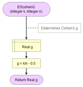
It takes as input the frequency of one of the categories (k) and the sample size (n).
Flowgorithm file: ES - Cohen g.fprg.
with Python
Jupyter Notebook from video: ES - Cohen g.ipynb.
Datafile used in video: StudentStatistics.csv
with R (Studio)
R script from video: binary - effect sizes.R.
Datafile used in video: StudentStatistics.sav
with SPSS
Datafile used in video: StudentStatistics.sav
Online calculator
Enter the number of cases of the first category, then the total sample size:
Manually (using Formula)
Given a sample proportion (p) and the expected proportion in the population (π), the formula for Cohen's g will be:
\(g=p-\pi\)
The sample proportion in the example was 0.26 and the expected proportion was 0.50, in the example this therefor gives:
\(g=0.26-0.50=-0.24\)
Often the absolute value is used (the so-called nondirectional Cohen's g):
\(g=|0.26-0.50|=|-0.24|=0.24\)
The last step is to report the results. This will be discussed in the next section.
Appendix
Alternative Ratio/Relative Risk (click to expand)
The Alternative Ratio is only mentioned in the documentation of a program called PASS (NCSS, n.d.), and referred to as Relative Risk by JonB (2015). Relative Risk is more often used with cross tables, so I’ll stick with the ‘Alternative Ratio’. It is simply the sample proportion (percentage), divided by the expected population proportion (which we set at 0.5 (50%)). In the example the sample proportion of the female was 0.26, and dividing this by 0.5 gives an Alternative Ratio of 0.26 / 0.5 = 0.52. This means that the female proportion was (1 – 0.52) = 48% lower than expected. Similar for the male we get 0.74 / 0.5 = 1.48. This indicates that the male proportion is 48% higher than expected. Unfortunately, there is no rule to determine if 48% is high or low (although most people would find it pretty high).
Click here to see how to determine the Alternative Ratio...
with Flowgorithm
A basic implementation for the Alternative Ratio is shown in the flowchart in figure 1
Figure 1
Flowgorithm for the Alternative Ratio
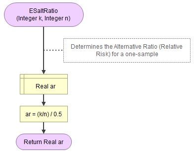
It takes as input the frequency of one of the categories (k) and the sample size (n).
Flowgorithm file: ES - Alternative Ratio.fprg.
with Python
Jupyter Notebookfrom video: ES - Alternative Ratio.ipynb.
Datafile used in video: StudentStatistics.csv
with R
The Jupyter notebook used in the video: ES - Alternative Ratio.ipynb
The data file used: StudentStatistics.sav
R Studio file: ES - Alternative Ratio.R
with SPSS (not directly possible)
Unfortunately I'm not aware of any method to determine the Alternative Ratio with SPSS. However, it is fairly easy to determine the frequencies for each category and use the online calculator below to determine the Alternative Ratio.
Datafile used: StudentStatistics.sav
Online calculator
Enter the number of cases in the category of interest, then the total sample size, and the expected proportion (usually 0.5 for binary data):
Manually (with Formula)
Given a sample proportion (p) and the expected proportion in the population (π), the formula for the Alternative Ratio (Relative Risk) will be:
\(AR=\frac{p}{\pi}\)
In the example the sample proportion of female was 0.26 and the expected proportion in the population 0.50. Filling this in the formula yields:
\(AR=\frac{0.26}{0.5}=0.52\)
And for the male proportion, which was 0.74 in the sample, we get:
\(AR=\frac{0.74}{0.5}=1.48\)
Cohen’s h2 (click to expand)
Click here if you prefer to watch a video on the explanation of Cohen's h2
Cohen’s h2 looks at the difference between two proportions. However, it does not consider the difference of the two sample proportions directly, but rather the arcsin transformations of their square root. Cohen explains that although 0.65 and 0.45 have the same difference as 0.25 and 0.05, the power of these two is actually different. To compensate for this a non-linear transformation is used and the arcsin seems to do the trick. For more info see page 180 & 181.
Note that Cohen's h is slightly different from Cohen's h2. The general Cohen's h is used for so-called paired samples, not for a one-sample scenario, like a binomial test. For the interpretation Cohen gives guidelines for only Cohen's h, not h2, but does give a conversion on page 203:
$$h=h_2\times\sqrt{2}$$
The interpretation of h can then be done using (adapted from Cohen (1988, p. 198)) :
| Cohen’s h | Interpretation |
|---|---|
| 0.00 < 0.20 | Negligible |
| 0.20 < 0.50 | Small |
| 0.50 < 0.80 | Medium |
| 0.80 or more | Large |
| Note: Adapted from Statistical power analysis for the behavioral sciences (2nd ed., p. 198) by J. Cohen, 1988, L. Erlbaum Associates. | |
Click here to see how to determine Cohen's h2...
with Excel
Excel file used: ES - Cohen h2.xlsm
with Flowgorithm
A basic implementation for Cohen Cohen's h2 is shown in the flowchart in figure 1
Figure 1
Flowgorithm for Cohen h2
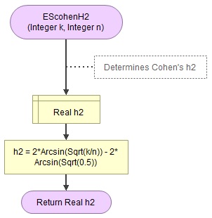
It takes as input the frequency of one of the categories (k) and the sample size (n).
Flowgorithm file: ES - Cohen h2.fprg.
with SPSS
Data file used: StudentStatistics.sav
Online calculator
Enter the number of 'successes' (or number of respondents of the first category, the total sample size, and the expected proportion:
Manually (using formula)
The formula for Cohen's h2 will be:
\(h_2=\phi_{1}-\phi_{c}\)
Where φi is determined by:
\(\phi_{i}=2\times\textup{arcsin}\sqrt{p_{i}}\)
Where pi is the sample proportions of category i, arcsin the inverse sinus function (also known as sin-1), and pc the expected proportion
In the example the female proportion is approximately 0.2609, filling this in for phi (φ) gives:
\(\phi_{1}=2\times\textup{arcsin}\sqrt{0.2609}\approx1.0722\)
For the expected proportion, which was 0.50 we get:
\(\phi_{c}=2\times\textup{arcsin}\sqrt{0.50}\approx1.5708\)
Filling these results in the formula for Cohen's h2 we get:
\(h_2\approx1.0722-1.5708\approx-0.4986\)
And just for the interpretation, converting this to Cohen's h we get:
\(h\approx-0.4986\times\sqrt{2}\approx-0.7051\)
Single binary variable
![]()

Google adds