
Analysing a single nominal variable
Part 3c: Effect size (Cramér's V and Relative Risks)
In the previous part we saw that all percentages in the example were different from each other. However if a sample size is large enough any minor difference will still result in a significant result. For this it is recommended to also add a so-called effect size.
We can determine an effect size for the overall test (the Pearson chi-square), and also for the pairwise comparisons (the binomial tests).
Effect size for the overall test
Note: click here if you prefer to watch a video
A possible effect size for the very first test we did (the omnibus test known as Pearson Chi-square test) is Cramér's V (Cramér, 1946). This measure is actually designed for the chi-square test for independence but can be adjusted for the goodness-of-fit test (Kelley & Preacher, 2012, p. 145; Mangiafico, 2016, p. 474). It gives an estimate of how well the data then fits the expected values, where 0 would indicate that they are exactly equal. If you use the equal distributed expected values (as we did in the example) the maximum value would be 1, otherwise it could actually also exceed 1.
As for the interpretation for Cramér's V various rules of thumb exist. Cohen offers an interpretation for his w (Cohen, 1988, p. 227), and this w can be converted to Cramérs V using:
\(V=\frac{w}{\sqrt{k-1}}\)
Cohen used w = 0.10 for small, 0.30 for medium and 0.5 for large. Using the formula we can convert these to thresholds for Cramér's V, which will then depend on the number of categories (k). In table 1 the first few are shown.
| k | Negligible | Small | Medium | Large |
|---|---|---|---|---|
| 2 | 0 < 0.100 | 0.100 < 0.300 | 0.300 < 0.500 | ≥ 0.500 |
| 3 | 0 < 0.071 | 0.071 < 0.212 | 0.212 < 0.354 | ≥ 0.354 |
| 4 | 0 < 0.058 | 0.058 < 0.173 | 0.173 < 0.289 | ≥ 0.289 |
| 5 | 0 < 0.050 | 0.050 < 0.150 | 0.150 < 0.250 | ≥ 0.250 |
| k | 0.1 / SQRT(k-1) | 0.3 / SQRT(k-1) | 0.5 / SQRT(k-1) | |
| Note: Adapted from Statistical power analysis for the behavioral sciences (2nd ed., pp. 227) by J. Cohen, 1988, L. Erlbaum Associates. | ||||
The last row shows how you can determine the upper limits for each classification for any number of categories (k)
In the example Cramér's V is 0.401 (see videos below on how to determine this), and we had 5 categories, which would indicate a large effect.
We could add this to our report:
A chi-square test of goodness-of-fit was performed to determine whether the marital status were equally chosen. The marital status was not equally distributed in the population, χ2(4, N = 1941) = 1249.13, p < .001, with a relatively strong (Cramér's V = .40) effect size according to conventions for Cramér's V (Rea & Parker, 1992).
Click here to see how to obtain Cramér's V.
with Excel
Excel file from video: ES - Cramers V (GoF).xlsm.
with Flowgorithm
A basic implementation for Cramér's V in the flowchart in figure 1
Figure 1
Flowgorithm for Cramér's V
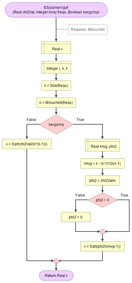
It takes as input the chi-square value, an array of integers with the observed frequencies, and a boolean to indicate to use the Bergsma correction.
It uses a small helper function to sum an array of integers.
Flowgorithm file: FL-EScramerVgof.fprg.
with Python
Jupyter Notebook from video: ES - Cramers V (GoF).ipynb.
Data file from video: GSS2012a.csv.
with R (Studio)
R script from video: ES - Cramers V (GoF).R.
Data file from video: Pearson Chi-square independence.csv.
Jupyter Notebook: ES - Cramers V (GoF) (R).ipynb.
with SPSS
Unfortunately SPSS does not have a method to determine Cramér's V directly from the GUI, however the calculation is not very difficult once you have the output from the previous part.
The video below shows how this could be done with a bit of help from Excel
Online calculator
Enter the requested information below:
Manually (formula and example)
Formula
The formula for Cramér's V is:
\(V=\sqrt\frac{\chi^{2}}{n\times df}\)
In the above formula \(\chi^2\) is the chi-square test value, \(n\) is the total sample size, and \(df\) is the degrees of freedom, determined by \(df=k-1\). \(k\) is the number of categories.
Example.
If we have a chi-square value of 1249.13, a total sample size of 1941, and had five categories, we can first determine the degrees of freedom (df):
\(df = k - 1 = 5 - 4 = 4\)
Then we can fill out all values in the formula for Cramér's V:
\(V=\sqrt\frac{\chi^{2}}{n\times df}=\sqrt\frac{1249.13}{1941\times4}=\sqrt\frac{1249.13}{7764}\approx\sqrt{0.1609}\approx0.4011\)
A correction can be applied using the procedure proposed by Bergsma (2013). This is actually for a Cramér’s V with a chi-square test of independence, but adapting it for a goodness-of-fit is possible.
Alternatives for Cramér's V as an effect size measure can also be Cohen's w, or Johnston-Berry-Mielke E.
Click here to see how to obtain Cohen's w
with Excel
Excel file from video: ES - Cohen w.xlsm.
with Flowgorithm
A basic implementation for Cohen's w in the flowchart in figure 1
Figure 1
Flowgorithm for Cohen's w
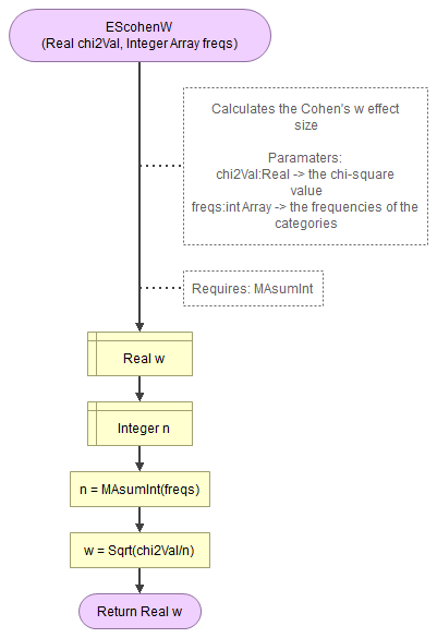
It takes as input the chi-square value, an array of integers with the observed frequencies.
It uses a small helper function to sum an array of integers.
Flowgorithm file: FL-EScohenW.fprg.
with R (studio)
R script from video: ES - Cohens w.R.
Data file from video: GSS2012a.csv.
Jupyter Notebook: ES - Cohen w (R).ipynb.
with SPSS (not possible?)
To my knowledge it is not possible to determine Cohen's w with SPSS. However, SPSS does return the chi-square value and sample size, so you can use those values with the online calculator below to determine Cohen's w.
Online Calculator
Formula
\(w=\sqrt\frac{\chi^{2}}{n}\)
In the above formula \(\chi^2\) is the chi-square test value, \(n\) is the total sample size, and \(k\) is the number of categories.
Given Cramer's V (\(V\)) and the number of categories (\(k\)), the formula for Cohen's w will be:
\(w=V\times\sqrt{k-1}\)
Click here to see how to obtain Johnston-Berry-Mielke.
with Excel
Excel file from video: ES - JBM E.xlsm.
with Flowgorithm
A basic implementation for Johnston-Berry-Mielke E in the flowchart in figure 1
Figure 1
Flowgorithm for Johnston-Berry-Mielke E
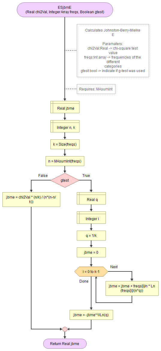
It takes as input the chi-square value, an array of integers with the observed frequencies, and a boolean to indicate if the g-test was used.
It uses a small helper function to sum an array of integers.
Flowgorithm file: FL-ESjbmE.fprg.
with R
R Script from video: ES - JBM E.R.
Data file from video: GSS2012a.csv.
Jupyter Notebook: ES - JBM E (R).ipynb.
Formula
Johnston-Berry-Mielke E (for Pearson chi-square, and for likelihood ratio):
(from Johnston, Berry, and Mielke (2006).
\(E_{\chi^2}=\frac{q}{1-q}\times \sum_{i=1}^{k}\left(\frac{p_{i}^{2}}{q_{i}}-1\right)\)
\(E_{L}=-\frac{1}{\textup{ln}(q)}\times\sum_{i=1}^{k}\left(p_{i}\times\textup{ln}\left(\frac{p_{i}}{q_{i}}\right)\right)\)
In the above formula's \(p_i\) is the observed proportion in category \(i\), \(q_i\) is the expected proportion in category \(i\), \(q\) the minimum of all \(q_i\)'s, and \(k\) the number of categories.
Effect size for the pairwise tests
For the pairwise comparisons we did with any of the effect sizes mentioned at the binomial test (see here) can be used: Cohen's h2, Cohen's g, and Alternative Ratio (Relative Risk) (JonB, 2015). In the example I'll use Relative Risk, which tells how many times more likely than was expected a category was chosen compared to the other.
In the example the Relative Risks ranged from 1.11 (divorced vs. never married) to 1.85 (married vs. seperated). Which we can also add to our report:
The binomial test pairwise comparison with Bonferroni correction of marital status showed that all proportions were significantly different from each other (p < .003). The Relative Risks ranged from 1.11 (divorced vs. never married) to 1.85 (married vs. seperated).
Click here to see how to obtain Effect Sizes pairwise.
with Excel (RR)
Excel file: ES - Alternative Ratio (pairwise).xlsm.
with Python
Jupyter Notebook from video: ES - Pairwise GoF.ipynb.
Data file from video: GSS2012a.csv.
with R (RR)
R script: ES - Alternative Ratio (pairwise).R.
Data file from video: Pearson Chi-square independence.csv.
not possible with SPSS
Unfortunately the GUI of SPSS does not have a way to determine Relative Risks from a binomial test.
Now we have fully analyzed our nominal variable. In the next part we combine all the reports section to create a final example of how you could report all the findings.
Single nominal variable
![]()

Google adds