
Binary vs. Binary (unpaired/independent)
Effect Size
The test only informs us if there is a significant association, but not how strong this association is. For that, we need an effect size measure. For the Fisher Exact test, the effect size that is often used is the Odds Ratio (OR).
Odds can sometimes be reported as 'a one in five odds', but sometimes as 1 : 4. This later notation is less often seen, but means for every one event on the left side, there will be four on the right side.
The Odds is the ratio of that something will happen, over the probability that it will not. There were 8 out of 11 female students who had their secondary school in 'The Netherlands', and 3 out of 11 who had it somewhere else. So the odds are: (8/11) / (3/11) = 8/3
For the Odds Ratio, we compare this with the second group, the males. For them the odds was 16/15. The odds ratio is therefor (8/3) / (16/15) = (8*15) / (3*16) = 5/2
Click here to see how to obtain the Odds Ratio.
with Flowgorithm
A basic implementation for the Odds Ratio is shown in figure 1
Figure 1
Flowgorithm Odds Ratio

It takes as input the four cell values
Flowgorithm file: FL-ESoddsRatio.fprg.
with Python
video to be uploaded
Jupyter Notebook from video: ES - Odds Ratio.ipynb.
Data file: StudentStatistics.csv.
with SPSS
video to be uploaded
Manually (formula and example)
Formula
If we are given a 2 by 2 table, and label each cell as shown in Table 1.
| Col. 1 | Col. 2 | |
|---|---|---|
| Row 1 | a |
b |
| Row 2 | c |
d |
The formula for the Odds Ratio is then:
\(OR=\frac{\left(\frac{a}{c}\right)}{\left(\frac{b}{d}\right)} = \frac{a\times d}{b\times c}\)
Example
The 2x2 table from the example.
| Female | Male | |
|---|---|---|
| The Netherlands | 8 |
16 |
| Other | 3 |
15 |
The formula for the Odds Ratio is then:
\(OR=\frac{\left(\frac{8}{3}\right)}{\left(\frac{16}{15}\right)} = \frac{8\times 15}{16\times 3} = \frac{5}{2} \)
If the result is 1, it indicates that gender has no influence on secondary school. A result higher than 1, indicates the odds are higher for Male than for Female to have secondary school in "other". A result lower than 1, indicates the odds are lower for male than for female to have secondary school in "other"
There are different rules of thumb as to classify a particular OR as small, medium or high. There are also often those who frown upon the use of these rules of thumb, and argue that it depends on the data you are working with. One rule of thumb would be from Wuensch (2009), shown in Table 1.
| OR | Interpretation |
|---|---|
| 1 < 1.5 | negligible |
| 1.5 < 3.5 | small |
| 3.5 < 9 | medium |
| 9 or more | large |
| Note: Adapted from Cohen’s conventions for small, medium, and large effects by K. Wuensch, 2009. | |
Jones (2014) finds the values a bit on the high end, and mentions he has seen rules of thumb as shown in Table 2. These are probably by taking the values Cohen proposes for Cohen's d, and using a conversion from Chinn (2000). Chinn proposes to use \(d = \frac{\text{ln}\left(OR\right)}{1.81}\), from this we can rewrite \(OR = e^{1.81\times d} \). Using this formula and Cohen's thresholds of 0.2, 0.5, and 0.8, the results are close to the ones shown in Table 2.
| OR | Interpretation |
|---|---|
| 1 < 1.5 | negligible |
| 1.5 < 2.5 | small |
| 2.5 < 4.3 | medium |
| 9 or more | large |
| Note: Adapted from How do you interpret the odds ratio (OR)? by J. Kelvyn, 2014. | |
In the example, we had an effect size (OR) of 5/2. This 2.5 could therefor be considered a small effect size (using table 1), or just at medium (using table 2). If your effect size is less than 1, you can calculate the Odds Ratio from the other categories perspective. In the example the odds ratio of 5/2 was obtained, since we had "The Netherlands" as the first row. If we had switched the two rows, it would have resultated in an Odds Ratio of 2/5. The same can be achieved by swopping the two columns.
Besides the Odds Ratio, there are many other measures we could also use. Including the so-called tetrachoric correlations.
Click here for more info on other binary-binary association measures
Click here to see a video instead of reading.
After performing chi-square test the question of the effect size comes up. An obvious candidate to use in a measure of effect size is the test statistic, the χ^2. One of the earliest and often mentioned measure uses this: the phi coefficient (or mean square contingency). Both Yule (1900) and Pearson (1900)mention this measure, and Cole (1949) refers to it as Cole C4. It is interesting that this gives the same result, as if you would assign a 0 and 1 to each of the two variables categories, and calculate the regular correlation coefficient.
This measure is also sometimes used for larger tables, but the range of values it can hold depends then on the size of the table. To overcome this an alternative was proposed by Pearson (1904): the contingency coefficient. This will range between 0 and 1, but the real maximum still depends on the size of the table.
Cole (1949) noted that for a 2x2 table the maximum would be √(1/2) and we prefer to have a correlation have a maximum of 1. Cole C5 does this by simply taking the contingency coefficient and dividing it by the √(1/2).
Another approach is by realizing that if there is no association, all cells have the same value, i.e. a = b = c = d. We can also write this as:
\(a=\frac{\left(a+b\right)\times\left(a+c\right)}{n}\)
The Forbes Coefficient (Forbes, 1907) uses this. This has a value of 1 if there is no association, while it has a value of 0 or 2 when there is a perfect one.
To adjust to the more traditional range of -1 to 1, Cole 1 simply subtracts one from the Forbes coefficient.
Another range of measures employ the Odds Ratio. Edwards (1963) argued that a measure of association for a 2x2 table should be some function of the cross-ratio bc/ad (e.g. the Odds Ratio).
Yule Q and Yule Y do exactly that. They are both of the format of:
\(\frac{OR^x-1}{OR^x-1}\)
Yule Q actually looks at the difference between the number of pairs that are in agreement and those in disagreement, and then divides this over the total possible number of pairs.
Click for more details on Yule's Y
If we have a 2 by 2 table, and one of the diagonals is zero, there would be a perfect association. For example:
| Column 1 | Column 2 | |
|---|---|---|
| Row 1 | 5 | 0 |
| Row 2 | 0 | 5 |
In contrast, if all the values would be the same, there wouldn't be any association:
| Column 1 | Column 2 | |
|---|---|---|
| Row 1 | 5 | 5 |
| Row 2 | 5 | 5 |
How about a table where the diagonals have the same values. For example:
| Column 1 | Column 2 | |
|---|---|---|
| Row 1 | 3 | 5 |
| Row 2 | 5 | 3 |
In this case, we can split the table into two tables, such that the sum of the two tables would add up to the original. The split is made in such a way that one has a perfect association, while the other is then having no association at all.
| Column 1 | Column 2 | |
|---|---|---|
| Row 1 | 0 | 2 |
| Row 2 | 2 | 0 |
| Column 1 | Column 2 | |
|---|---|---|
| Row 1 | 3 | 3 |
| Row 2 | 3 | 3 |
The sum of all counts in the perfect association part is 0+2+2+0=4, while for the no association part we get 3+3+3+3=12. Overall, we have 4/(4+12) = 4/16 = 25% of perfect association.
Notice that we can use the following formula in case of a table with the same diagonal:
\(\frac{a-b}{a+b}\)
If we apply this to our table 1, we get a nice value of 1, in table 2 a value of 0 and in table 3 a value of -0.25. This however, only works if each of the diagonals has the same values.
Unfortunately though, most tables don't have the same values across their diagonal. However, we can transform any table into a table with the same Odds Ratio, which is then symmetrical. This can be done by setting:
\(a = d = \sqrt{OR}, b = c = 1\)
Lets have a look at an example:
| Column 1 | Column 2 | |
|---|---|---|
| Row 1 | 3 | 15 |
| Row 2 | 8 | 16 |
We first determine the Odds Ratio of this table:
\(OR = \frac{a\times d}{b\times c} = \frac{3\times 16}{15\times 8} = \frac{48}{120} = \frac{2}{5}\)
We now use the suggestion: \(a = d = \sqrt{OR}, b = c = 1\), to create a table with the same Odds Ratio, but that has the diagonals the same:
| Column 1 | Column 2 | |
|---|---|---|
| Row 1 | \(\sqrt{\frac{2}{5}}\) | 1 |
| Row 2 | 1 | \(\sqrt{\frac{2}{5}}\) |
If you like, you can double check to see if the Odds Ratio of Table 6 is still \(\frac{2}{5}\)
Since Table 6 has the same values on the diagonals, we can apply our formula from earlier:
\(\frac{a-b}{a+b} = \frac{\sqrt{\frac{2}{5}}-1}{\sqrt{\frac{2}{5}}+1}\approx -0.225\)
So about 23% of a perfect association. Yule's Y does all these steps for us in one go, and will then of course produce the same result:
\(Y = \frac{\sqrt{a\times d}-\sqrt{b\times c}}{\sqrt{a\times d}+\sqrt{b\times c}} \approx -0.225\)
Unfortunately if any of the four cells is 0, the association will always return a 1 or -1. Similar if one or two cells have very high counts and the others very few, the result might be close to 1 or -1, even though there is almost no association. This is the same problem as for Yule's Q and the reason why Michael and McEwen developed their variation on Yule's Q.
For Yule Q the \(x=1\) and for Yule Y \(x=0.5\). Digby (1983, p. 754) showed that Yule’s Q consistently overestimates the association, while Yule’s Y underestimates it It seems that a better approximation might be somewhere between 0.5 and 1 as the power to use on the Odds Ratio. Digby H found the best result at 0.75, while Edwards (1957 as cited in Becker & Clogg, 1988, p. 409) had proposed π/4 (appr. 0.79).
Bonett and Price Y* uses a function to determine what the power should be (Bonett & Price, 2007).
A problem with all of Forbes and OR based is that the if only one cell is very large compared to the others, or if one cell is 0 the association will be quite large (close to -1 or 1).
Michael (1920, p. 55) worked together with McEwen and tried to overcome this with the 'McEwen and Michael coefficient'. Cole however criticized Michael a bit on this, that although at first one might not consider the example table a strong association, with so little data, there are actually very few other value arrangements with the same marginal totals, that would have yielded a stronger association. He states: “with any given series of collections containing two species the possible number of tables yielding different values for the number of joint occurrences is exactly one more than the smallest of the four marginal totals” (Cole, 1949, p. 417).
Cole C7 attempts to overcome this problem. Cole suggested to divide the absolute difference of deviation from no association by the number of possible tables with a positive association. He called this the coefficient of interspecific association
Another category are the tetrachorical correlations. In essence this attempts to mimic a correlation coefficient between two scale variables. It can be defined as "An estimate of the correlation between two random variables having a bivariate normal distribution, obtained from the information from a double dichotomy of their bivariate distribution" (Everitt, 2004, p. 372).
This assumes the two binary variables have ‘hidden’ underlying normal distribution. If so, the combination of the two forms a bivariate normal distribution with a specific correlation between them. The quest is then to find the correlation, such that the cumulative density function of the z-values of the two marginal totals of the top-left cell (a) match that value.
This is quite tricky to do, so a few have proposed an approximation for this. These include Yule r, Pearson Q4 and Q5, Camp, Becker and Clogg, and Bonett and Price.
Besides closed form approximation formula's, various algorithms have been designed as well. The three most often mentioned are Brown (1977), Kirk (1973), and Divgi (1979).
Click here on how to calculate each of the measures
with Flowgorithm
The Flowgorithm of the versions listed below were all included in one file, except for Brown's approximation, and Kirk's approximation:
Flowgorithm file: FL-ESbinBinAssociation.fprg.
See the section of Brown, and Kirk for the link to their approximation Flowgorithm files.
Becker and Clogg (1988)
Bonett and Price (2005)

Camp (1934)

Cole (1949)
Cole C1:

Cole C2, see Yule's (= Pearson's Phi) (1920)
Cole C3, see McEwen and Michael (1920)
Cole C4, see Yule's Q (= Pearson Q 2) (1900)
Cole C5:

Cole C6, see Pearson Q 3 (1900)
Cole C7:

Digby (1983)

Divgi (1979)
Edwards (1957)

Forbes (1907)


McEwen and Michael (1920)
same as Cole C3:

Pearson (1900)
Pearson Q1:

Pearson Q2, see Yule's Q (1900)
Pearson Q3 (= Yule's r, Cole's C6):

Pearson Q4:

Pearson Q5:
Yule's Q and Phi(1900)
Yule's Q (= Pearson's Q2, Cole's C4:

Yule's Phi = Pearson's Phi:

Yule's r see Pearson Q3 (1900)
Yule's Y (1912)

with Formula's
Yule Q (1900) (= Cole C4, and Pearson Q2)
Yule's Q (Yule, 1900, p. 272) can be calculated using:
\(Q = \frac{a\times d - b\times c}{a\times d + b\times c}\)
As for the interpretation for Q, there aren't many rules of thumb I could find. One I did find is from Glen (2017):
| |Q| | Interpretation |
|---|---|
| 0 < 0.30 | negligible |
| 0.30 < 0.50 | small |
| 0.50 < 0.70 | medium |
| 0.70 or more | large |
| Note: Adapted from Gamma Coefficient (Goodman and Kruskal's Gamma) & Yule's Q by S. Glen, 2017. | |
Alternative, the Q can be converted to an Odds Ratio and in turn, some proposed to convert an Odds Ratio to Cohen's d. Also Cohen's d can be calculated to a correlation coefficient (r), for which again there are different tables.
\(OR = \frac{1 + Q}{1 - Q}\)
Pearson Phi Coefficient (1900) (= Yule Phi Coefficient = Cole C2)
Pearson Phi Coefficient (Pearson, 1900, p. 12) is not a tetrachoric correlation, but rather the 'standard' correlation if you would give each of the two values for each of the two variables a 0 and 1. Yule also derived the same result (Yule, 1912, p. 596). The formula can be written as:
\(\phi = \frac{a\times d - b\times c}{\sqrt{R_1\times R_2\times C_1\times C_2}}\)
The formula can also be re-written to use the Pearson chi-square statistic , Cole's C2 (1949) uses this:
\(C_2 = \sqrt{\frac{\chi^2}{n}}\)
Cohen (1988, p. 216) refers to this as 'w'. He uses the proportions in the cross table and gives the equation:
\(w = \sqrt{\sum_i\sum_j\frac{\left(p_{ij} - \pi_{ij}\right)^2}{\pi_{ij}}}\)
Where \(\pi_{ij}\) is the expected proportion for cell row i column j, and \(p_{ij}\) the sample proportion.
Cohen also provided some guidelines for the interpretation:
| phi | Interpretation |
|---|---|
| 0 < 0.10 | negligible |
| 0.10 < 0.30 | small |
| 0.30 < 0.50 | medium |
| 0.50 or more | large |
| Note: Adapted from Statistical power analysis for the behavioral sciences by J. Cohen, 1988, pp. 224-225. | |
Pearson Q1 (1900)
Pearson Q1 (Pearson 1900, p. 15)
\( Q_1 = \sin\left(\frac{\pi}{2} \times \frac{a\times d - b\times c}{\left(a+b\right)\times\left(b+d\right)}\right) \)
Note that Pearson (1900) stated: "Q1 was found of little service" (p. 16).
Forbes Coefficient (1907)
Forbes Coefficient (1907, p. 279)
\( F=\frac{n\times a}{\left(a+b\right)\times\left(a+c\right)} \)
Cole (1949) later adjusted this to range from -1 to 1 and dubbed it C1.
Yule Y (1912)
Yule's Y (1912, p. 592) is a further adaptation of Yule's Q into:
\(Y = \frac{\sqrt{a\times d} - \sqrt{b\times c}}{\sqrt{a\times d} + \sqrt{b\times c}}\)
Yule referred to this as referred to as the coefficient of colligation.
The Odds Ratio can also be calculated from this using:
\(OR = \left(\frac{Y + 1}{1 - Y}\right)^2\)
Tables for the interpretation of the Odds Ratio can then be used.
McEwen and Michael (1920) (= Cole C3)
Michael (1920, p. 55) worked together with McEwen and named the following 'McEwen and Michael coefficient':
\(\frac{a\times d - b\times c}{\left(\frac{a+ d}{2}\right)^2 + \left(\frac{b+ c}{2}\right)^2}= \frac{4\times\left(a\times d - b\times c\right)}{\left(a+d\right)^2+\left(b+c\right)^2}\)
Later Cole (1949, p. 415) rewrote this equation for his C3 into:
\(C_3 = \frac{4\times\left(a\times d - b\times c\right)}{\left(a+d\right)^2+\left(b+c\right)^2}\)
Cole C1 (1949)
Cole's C1(1949, p. 415) is an adjusted Forbes Coefficient to:
\( C_1=\frac{a\times d - b\times c}{\left(a+b\right)\times\left(a+c\right)} \)
Cole C5 (1949)
Cole's C5 (1949, p. 416) is an adjustment of the Contingency Coefficient for 2x2 tables:
\( C_5 = \frac{\sqrt{2}\times\left(a\times d-b\times c\right)} {\sqrt{\left(a\times d-b\times c\right)^2 + R_1\times R_2\times C_1\times C_2}} \)
Cole C7 (1949)
Cole's C7 (1949, pp. 420-421) is the measure Cole derived himself and calls it 'coefficient of interspecific association" given as:
\(\frac{a\times d - b\times c}{\left(a+b\right) \times \left(b + d\right)}\)
Edwards Q (1957)
Edwards Q (1957, p. ???) as a variation on Yule's Q:
\( Q_E = \frac{OR^{\pi/4} - 1}{OR^{\pi/4} + 1} \)
\(OR=\frac{\left(\frac{a}{c}\right)}{\left(\frac{b}{d}\right)} = \frac{a\times d}{b\times c}\)
Digby H (1983)
Digby's H (1983, p. 754)
\(H = \frac{\left(a\times d\right)^{3/4} - \left(b\times c\right)^{3/4}}{\left(a\times d\right)^{3/4} + \left(b\times c\right)^{3/4}}\)
Bonett and Price Y* (2007)
Bonett and Price (2007, pp. 433-434)
\(Y* = \frac{\hat{\omega}^x-1}{\hat{\omega}^x+1}\)
With:
\(x = \frac{1}{2}-\left(\frac{1}{2}-p_{min}\right)^2\)
\(p_{min} = \frac{\text{MIN}\left(R_1, R_2, C_1, C_2\right)}{n}\)
\(\hat{\omega} = \frac{\left(a+0.1\right)\times\left(d+0.1\right)}{\left(b+0.1\right)\times\left(c+0.1\right)}\)
Note that \(\hat{\omega}\) is a biased corrected version of the Odds Ratio.
Alroy's Forbes Adjustment (2015)
Alroy adjusts the Forbes coefficient by setting (Alroy, 2015):
\(F' = \frac{a\times\left(n' + \sqrt{n'}\right)}{a\times\left(n' + \sqrt{n'}\right) + \frac{3}{2}\times b\times c}\)
With:
\(n' = a + b + c\)
Alroy refers to the Forbes coefficient as a measure of similarity. Alroy then sets out to improve the measure by disregarding the lower left value (d).
Tetrachorical Correlation (approximations)
Yule's r (1900) (= Pearson Q3 = Cole C6)
Yule proposed to convert his Q to a correlation coefficient using (Yule, 1900, p. 276):
\(r_Q = \cos\left(\frac{\sqrt{k}}{1+\sqrt{k}}\times\pi\right)\)
\(k = \frac{1-Q}{1+Q}\)
Pearson's Q3 (1900) will give the same result, although he used the sinus function:
\(Q_2 = \sin\left(\frac{\pi}{2}\times\frac{\sqrt{a\times d} - \sqrt{b\times c}}{\sqrt{a\times d} + \sqrt{b\times c}}\right)\)
Cole (1949) rewrote this to:
\(C_6 = \cos\left(\frac{\pi\times\sqrt{b\times c}}{\sqrt{a\times d} + \sqrt{b\times c}}\right)\)
Pearson Q4 (1900)
Pearson Q4 (1900, p. 16)
\( Q_4 = \sin\left(\frac{\pi}{2} \times \frac{1}{1 + \frac{2\times b\times c\times n}{\left(a\times d -b\times c\right) \times \left(b+c\right)}}\right) \)
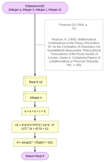
Pearson Q5 (1900)
Pearson Q5 (1900, p. 16)
\( Q_5 = \sin\left(\frac{\pi}{2} \times \frac{1}{\sqrt{1+ k^2}}\right) \)
with \( k^2 = \frac{4\times a\times b\times c\times d\times n^2}{\left(a\times d-b\times c\right)^2\times\left(a+d\right)\times\left(b+c\right)} \)
Becker and Clogg (1988)
Becker and Clogg (1988, pp. 410-412)
\( \rho^* = \frac{g-1}{g+1} \)
\( \rho^{**} = \frac{OR^{13.3/\Delta} - 1}{OR^{13.3/\Delta} + 1} \)
with:
\(g=e^{12.4\times\phi - 24.6\times\phi^3}\)
\(\phi = \frac{\ln\left(OR\right)}{\Delta}\)
\(OR=\frac{\left(\frac{a}{c}\right)}{\left(\frac{b}{d}\right)} = \frac{a\times d}{b\times c}\)
\(\Delta = \left(\mu_{R1} - \mu_{R2}\right) \times \left(v_{C1} - v_{C2}\right)\)
\(\mu_{R1} = \frac{-e^{-\frac{t_r^2}{2}}}{p_{R1}}, \mu_{R2} = \frac{e^{-\frac{t_r^2}{2}}}{p_{R2}} \)
\(v_{C1} = \frac{-e^{-\frac{t_c^2}{2}}}{p_{C1}}, v_{C2} = \frac{e^{-\frac{t_c^2}{2}}}{p_{C2}} \)
\(t_r = \Phi^{-1}\left(p_{R1}\right), t_c = \Phi^{-1}\left(p_{C1}\right)\)
\(p_{x} = \frac{x}{n}\)
\(\Phi^{-1}\left(x\right)\) is the inverse standard normal cumulative distribution function
\(OR\) is the Odds Ratio
Bonett and Price ρ* (2005)
Bonett and Price ρ* (2005, p. 216)
\(\rho^* = \cos\left(\frac{\pi}{1+\omega^c}\right)\)
With:
\(\omega = OR = \frac{a\times d}{b\times c}\)
\(c = \frac{1-\frac{\left|R_1-C_1\right|}{5\times n} - \left(\frac{1}{2}-p_{min}\right)^2}{2}\)
\(p_{min} = \frac{\text{MIN}\left(R_1, R_2, C_1, C_2\right)}{n}\)
Bonett and Price ρhat* (2005)
Bonett and Price ρhat* (2005, p. 216)
\(\hat{\rho}^* = \cos\left(\frac{\pi}{1+\hat{\omega}^\hat{c}}\right)\)
With:
\(\hat{\omega} = \frac{\left(a+\frac{1}{2}\right)\times \left(d+\frac{1}{2}\right)}{\left(b+\frac{1}{2}\right)\times \left(c+\frac{1}{2}\right)}\)
\(\hat{c} = \frac{1-\frac{\left|R_1-C_1\right|}{5\times \left(n+2\right)} - \left(\frac{1}{2}-\hat{p}_{min}\right)^2}{2}\)
\(\hat{p}_{min} = \frac{\text{MIN}\left(R_1, R_2, C_1, C_2\right)+1}{n+2}\)

Google adds