
Distributions
Chi-Square
The APA dictionary of Statistics and Research Methods defines the chi-square distribution as "a distribution of the sums of independent squared differences between the observed scores in a data set and the expected score for the set" (Zedeck, p. 43). It is an often encounted continuous distribution in statistics.
The 'chi' is the Greek letter χ , and with the 'square' it is therefor often written as χ2 (and 'chi' is therefor not pronounced as chi in 'thai chi').
The distribution depends on the so-called degrees of freedom (df). Four examples are shown of a chi-square distribution in figure 1.
Figure 1Examples of Chi-Square Distribution

Note that how higher the degrees of freedom, the more the distribution starts to look like a normal distribution.
The chi-square distribution is unlike the normal distribution, not symmetrical.
Also, we are often only interested in one tail of the chi-square distribution. Most often the distribution is used for a goodness-of-fit test. A left-tail would then indicate that the fit is too good, which shouldn't be a problem.
As with any continuous distribution it is very important to remember that we are usually only interested in the areas under the curve, since those give us the probability
Now calculating this area can be tricky business depending on how easy you want to make it on yourself
Use some software (easy)
to be uploaded
Use a chi-square distribution table (old school)
Unlike many other tables, the cells in a chi-square table will show the so-called 'critical' value, and not the p-value.
A table with the right-tail critical chi-square values is shown in Figure 2.
Figure 2Chi-Square Right Tail Critical Values

Suppose we have a chi-square value of 10.43 and a degrees of freedom of 4. We have set ourselves a 95% confidence level, i.e. alpha = 1 - 0.95 = 0.05
We look in the first column of the table, labelled 'df', to find our degrees of freedom of 4. Then we look for the column with our alpha of 0.05, and at the intersection we find 9.488.
Any chi-square value higher than 9.488 will have a p-value less than 0.05, and any value lower will have a p-value higher than .05.
Figure 3Chi-Square Right Tail Critical Values Example

In our example, the chi-square value of 10.43 is higher than our critical 9.488, so we could conclude this is significant at a .05 alpha level.
We could get an idea of what the p-value might be by looking for our chi-square value in the row of our df. The 10.43 fits between 11.143 and 9.488. These correspond to the column titles of 0.025 and 0.050. So, the p-value will be between .025 and .050.
We could use linear interpolation to get a rough approximation.
We have a range of critical values from 11.143 to 9.488, which is a length of 11.143 - 9.488 = 1.655. Our chi-square value of 10.43 is then 11.143 - 10.43 = 0.713 away, which is 0.713 / 1.1655 = 43% of the total range.
From the corresponding p-values the range is 0.05 - 0.025 = 0.025. 43% of this is 0.0108. We add this to the 0.025 and find a rough approximation of the p-value to be 0.0358.
The 0.0358 is fairly close to the result you would get with Excel of 0.0338
The calculations are visualised in Figure 4.
Figure 4Chi-Square Table Interpolation Visualisation
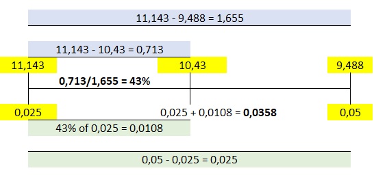
Start with filling out the yellow cells, then calculate the blue ones. Determine the percentage, and calculate the green cells. Finally determine the approximate p-value.
Use the formulas (hard core)
The probability density function of the chi-square distribution (the curve shown in Figure 1) is given by:
\( cpdf\left(x, k\right) = \frac{x^{\frac{k}{2} - 1}\times e^{-\frac{x}{2}}}{2^{\frac{k}{2}}\times\Gamma\left(\frac{k}{2}\right)} \)
Where \( x \) is usually the calculated \( \chi^2 \) value, and \( k \) is the degrees of freedom.
Since \( k \) is the degrees of freedom, it should be an integer. For the \( \Gamma \) function this gives as input \( \frac{k}{2} \) and with this we can define the function as:
\( \Gamma\left(a=\frac{x}{2}\right)=\begin{cases} \left(a - 1\right)! & \text{ if } x \text{ is even}\\ \frac{\left(2\times a\right)!}{4^a\times a!}\times\sqrt{\pi} & \text{ if } x \text{ is odd} \end{cases} \)
The cumulative distribution function is then simply the integral over the specified range:
\( ccdf\left(x, k\right) = \int_{i=0}^{x} cpdf\left(i,k\right) \)
As mentioned earlier we are usually interested in the right-tail, so simply subtracting the ccdf from 1 should give the desired result.
Calculating this integral is the most tricky part. This isn't a calculus course so I will not go into that. I will give two alternative methods to calculate this
Use bars to approximate
Lets say we have a chi-square value of 10.43 and 4 degrees of freedom. One method to approximate the size of the area under the curve, and with that the probability, is to split the area in multiple bars, as illustrated in figure 4.
Figure 4Chi-Square Table Interpolation Visualisation

Since the degrees of freedom is set to 4, we can already determine the denominator in the cpdf formula:
\( denom = 2^{\frac{k}{2}}\times\Gamma\left(\frac{k}{2}\right) \)
\( = 2^{\frac{4}{2}}\times\Gamma\left(\frac{4}{2}\right) \)
\( = 2^{2}\times\Gamma\left(\frac{4}{2}\right) \)
\( = 4\times\Gamma\left(\frac{4}{2}\right) \)
Determining the gamma function:
\( \Gamma\left(a=\frac{4}{2}\right)=\begin{cases} \left(2 - 1\right)! & \text{ if } 4 \text{ is even}\\ \frac{\left(2\times 2\right)!}{4^2\times 2!}\times\sqrt{\pi} & \text{ if } 4 \text{ is odd} \end{cases} \)
Since 4 is even we get:
\( \Gamma\left(a=\frac{4}{2}\right)=\left(2 - 1\right)! =1! = 1 \)
Plugging this back in to determine our denominator:
\( denom = 4\times 1 = 4 \)
So for this example we can simplify the cpdf formula to:
\( cpdf\left(x, 4\right) = \frac{x^{\frac{4}{2} - 1}\times e^{-\frac{x}{2}}}{4} \)
\( = \frac{x\times e^{-\frac{x}{2}}}{4} \)
Let's say we set the first bar from chi-square values 0 to 0.43, and use the lower value to determine the height, using the cpdf formula:
\( cpdf\left(0, 4\right) = \frac{0\times e^{-\frac{0}{2}}}{4} = \frac{0\times e^{0}}{4} = 0 \)
With a height of 0 and a width of 0.43 this first bar will have an area of 0.
The next bar will then be from chi-square values 0.43 to 0.93, and use the lower value to determine the height, using the cpdf formula:
\( cpdf\left(0.43, 4\right) = \frac{0.43\times e^{-\frac{0.43}{2}}}{4} \approx 0.0867 \)
With a height of 0.0867 and a width of 0.5 the second bar will have an area of 0.5 × 0.0867 = 0.04335
The third bar will then be from chi-square values 0.93 to 1.43, and use the lower value to determine the height, using the cpdf formula:
\( cpdf\left(0.93, 4\right) = \frac{0.93\times e^{-\frac{0.93}{2}}}{4} \approx 0.14604 \)
With a height of 0.14604 and a width of 0.5 the second bar will have an area of 0.5 × 0.14604 = 0.07302
We keep repeating these steps for the next bars:
\( cpdf\left(1.43, 4\right) = \frac{1.43\times e^{-\frac{1.43}{2}}}{4} \approx 0.17489 \)
\( cpdf\left(1.93, 4\right) = \frac{1.93\times e^{-\frac{1.93}{2}}}{4} \approx 0.18382 \)
\( cpdf\left(2.43, 4\right) = \frac{2.43\times e^{-\frac{2.43}{2}}}{4} \approx 0.18025 \)
\( cpdf\left(2.93, 4\right) = \frac{2.93\times e^{-\frac{2.93}{2}}}{4} \approx 0.16926 \)
\( cpdf\left(3.43, 4\right) = \frac{3.43\times e^{-\frac{3.43}{2}}}{4} \approx 0.15432 \)
\( cpdf\left(3.93, 4\right) = \frac{3.93\times e^{-\frac{3.93}{2}}}{4} \approx 0.1377 \)
\( cpdf\left(4.43, 4\right) = \frac{4.43\times e^{-\frac{4.43}{2}}}{4} \approx 0.12089 \)
\( cpdf\left(4.93, 4\right) = \frac{4.93\times e^{-\frac{4.93}{2}}}{4} \approx 0.10477 \)
\( cpdf\left(5.43, 4\right) = \frac{5.43\times e^{-\frac{5.43}{2}}}{4} \approx 0.08987 \)
\( cpdf\left(5.93, 4\right) = \frac{5.93\times e^{-\frac{5.93}{2}}}{4} \approx 0.07644 \)
\( cpdf\left(6.43, 4\right) = \frac{6.43\times e^{-\frac{6.43}{2}}}{4} \approx 0.06455 \)
\( cpdf\left(6.93, 4\right) = \frac{6.93\times e^{-\frac{6.93}{2}}}{4} \approx 0.05418 \)
\( cpdf\left(7.43, 4\right) = \frac{7.43\times e^{-\frac{7.43}{2}}}{4} \approx 0.04524 \)
\( cpdf\left(7.93, 4\right) = \frac{7.93\times e^{-\frac{7.93}{2}}}{4} \approx 0.0376 \)
\( cpdf\left(8.43, 4\right) = \frac{8.43\times e^{-\frac{8.43}{2}}}{4} \approx 0.03113 \)
\( cpdf\left(8.93, 4\right) = \frac{8.93\times e^{-\frac{8.93}{2}}}{4} \approx 0.02568 \)
\( cpdf\left(9.43, 4\right) = \frac{9.43\times e^{-\frac{9.43}{2}}}{4} \approx 0.02112 \)
\( cpdf\left(9.93, 4\right) = \frac{0.93\times e^{-\frac{0.93}{2}}}{4} \approx 0.01732 \)
Multiply each of the above with the width of 0.5, and then add all of them together to get....0.9609.
To get the right-tail, we simply subtract this from 1, to get 1 - 0.9609 = 0.0391. Which is the probability of getting a chi-square value of 10.43 or higher with df of 4. The more precise answer using Excel should have been 0.0338. So this approximation is pretty close. By making the bars even thinner, and/or using a trapezium we could have even gotten closer to the precise answer, but hopefully this gave an idea on how it could be done.
Use a numeric approximation
One possible numerical approximation is the ACM Algorithm 299 (Hill & Pike, 1966), which in turn uses ACM Algorithm 209 (Ibbetson, 1963) and is also used by Microsoft. The ACM 209 algorithm is for a normal distribution, and is discussed in that section. In figure 5 is a flow chart for ACM Algorithm 299.
Figure 5ACM 299 Flow Chart

Let's say we have a chi-square value (chi2) of 10.43 and degrees of freedom (df) of 4.
Starting at the top our chi2 is not 0 or less, and also our df is not below 1, so we move to the right and set the values as shown in the flow-chart, with \( a = 0.5 \times 10.43 = 5.215 \).
Our df of 4 is even, so we set 'even' to TRUE.
Since 4 is greater than 1, we set \(y = e^\left(-5.215\right) \approx 0.0054 \)
Next, since even is TRUE we also set \(s = y = 0.0054 \)
Since 4 is not less or equal to 2, we move to the right and set \( x = 0.5\times\left(4 - 1\right) = 0.5\times3 = 1.5 \)
even is TRUE so we move down and set \(z=1\).
Our \(a = 5.215\) which is less than 40, so we move to the right.
'even' is still TRUE, so move down and set \(ee=1\)
Moving down again we get \(c = 0\).
Since z = 1, and x = 1.5 our z-value is less or equal to x, so we move down
We set \(ee = 1\times\frac{5.215}{1} = 5.215 \), \(c = 0 + 5.215 = 5.125\), and \(z = 1 + 1 = 2\)
We now return and check that now z = 2 and x = 1.5. This time z is not less or equal to x, so we move to the right.
We set \(pVal = 5.215\times0.0054 + 0.0054 \approx 0.0338\)
Finally we return 1 - 0.0338 = 0.9662.
To get the right-tail, we simply subtract this from 1, to get 1 - 0.9662 = 0.0338. Which is the probability of getting a chi-square value of 10.43 or higher with df of 4. The same result as when using the Excel function.
Distributions
![]()

Google adds