
Distributions
Binomial distribution
The binomial distribution can be defined as: "the distribution of the number of ‘successes’, X, in a series of n independent Bernoulli trials where the probability of success at each trial is p and the probability of failure is q = 1 − p" (Everitt, 2004, p. 40). The Oxford Dictionary of Statistics (Upton & Cook, 2014, p. 43) defines it almost exactly the same. However, there are also those who define it as 'the probability distribution', rather than the absolute count distribution (Zedeck, 2014, p. 28; Porkess, 1991, p. 18).
The definition mentions Bernoulli trials, which can be defined as: "a set of n independent binary variables in which the jth observation is either a ‘success’ or a ‘failure’, with the probability of success, p, being the same for all trials" (Everitt, 2004, p. 35).
The classic example of Bernoulli trials (and for the binomial distribution) is flipping a coin. A coin flip is a binary variable, since there are only two possible outcomes (head or tail, ignoring that strickly speaking it might land on its side). We could define a 'success' as 'head' and if the coin is fair, the probability of success is 0.5. This probability will not change, and remains the same each time we flip the coin.
A Binomial Distribution would then be for example, flipping the coin 5 times and it will then show the probability of having 0, 1, 2, 3, 4, or 5 times a head. The binomial distribution depends on the number of trials (the sample size), usually denoted with n, and the probability of success on each trial, usually denoted with p.
The distribution will look different, depending on the number of trials and the probability of success.
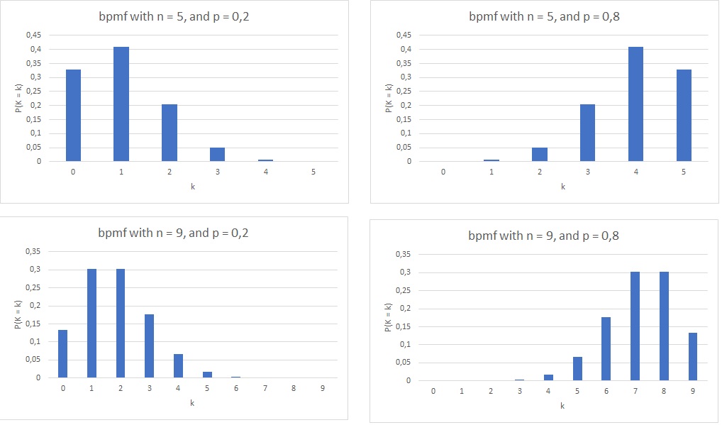
In figure 1 four examples are shown of the probability distribution of a binomial distribution (the binomial probability mass function (bpmf)).
Figure 1
Four Binomial pmf Examples
To find probabilities using the binomial distribution, there are three approaches.
Use some software (easy)
Excel
Python
Three different methods to use a binomial distribution with Python:
With Scipy Library
Jupyter Notebook: DI - Binomial (scipy).ipynb
With math Library
Jupyter Notebook: DI - Binomial (math).ipynb
Without libraries
Jupyter Notebook: DI - Binomial (core).ipynb
R
R script: DI - Binomial.R
SPSS
Use a binomial distribution table (old school)
Click here if you prefer to watch a video on this
In figure 2 a cumulative binomial distribution table
Figure 2
Cumulative Binomial Distribution Table

The table shows the probability of k or less successes. Lets use an example to illustrate how to work with it.
We have an unfair coin, where the probability of head is 0.8. We throw this coin 5 times and want to know the probability of at least twice a head.
The table columns for p only go up to 0.5, but this is not a problem. The probability of head is 0.8, which means that the probability for tail must be 1 - 0.8 = 0.2. And having at least twice a head, is the same as having at most 3 times a tail. So the probability for at least twice a head = the probability for at most 3 tails.
The number of trials is 5 (we throw the coin 5 times), so we look for the section where n = 5. Then within that section we look for our maximum number of succeses, the 3 (i.e. k = 3).
We finally select the column with our probability of success, the 0.2.
In figure 3 our selection is highlighted.
Figure 3
Cumulative Binomial Distribution Table Example
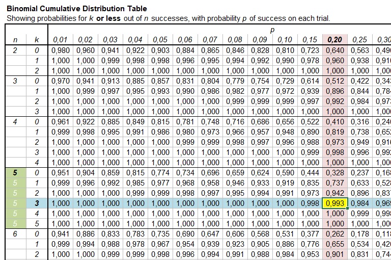
The intersection shows 0.993. This is the probability of 3 or less times a tail in five throws, if the chance of a tail is 0.2 each time. It is then also the probability of at least twice a head.
Use the formulas (hard core)
The formula for the count of the binomial distribution is given by the binomial coefficient:
\( \binom{n}{k}=\frac{n!}{k!(n-k)!} \)
This formula will tell us how many outcomes there are possible out of n, that have exactly k successes.
In this formula the \(!\) indicates the factorial operator defined as:
\( x! = \prod_{i=1}^x i = 1\times 2\times 3\times\dots\times\left(x-1\right)\times x\)
While the formula for the binomial probability distribution (the probability mass function) is given by:
\( bpmf(k,n,p)=\binom{n}{k}\times{p^k}\times(1-p)^{n-k} \)
This formula tells us the probability of exactly k successes in n trials, if the chance of success in each trial is p.
The cumulative binomial probability distribution (the cumulative distribution function) the formula is:
\( bcdf(k,n,p)=\sum_{i=0}^{\left\lfloor k\right\rfloor}\binom{n}{i}\times{p^i}\times\left(1-p\right)^{n-i} \)
This formula tells us the probability of k or less successes in n trials, if the chance of success in each trial is p. The brackets around the k in the sum, are the floor function, which means to round k down to the lowest integer. So if k would be 2.99 it would get rounded to 2.
worked out example
For example. We have an unfair coin, where the probability of head is 0.8. We throw this coin 5 times and want to know the probability of at least twice a head.
Note that at least twice head + less than twice head should equal 1, so at least twice head = 1 - less than twice head. Less than twice, is the same as 1 or less, and for this we can use the formula, with k=1, n=5 and p=0.8:
\( bcdf(1,5,0.8)=\sum_{i=0}^{\left\lfloor 1\right\rfloor}\binom{5}{i}\times{0.8^i}\times\left(1-0.8\right)^{5-i} \)
\( =\sum_{i=0}^{1}\binom{5}{i}\times{0.8^i}\times(0.2)^{5-i} \)
\( =\binom{5}{0}\times{0.8^0}\times(0.2)^{5-0} + \binom{5}{1}\times{0.8^1}\times\left(0.2\right)^{5-1} \)
\( =\binom{5}{0}\times{1}\times(0.2)^{5} + \binom{5}{1}\times{0.8}\times\left(0.2\right)^{4} \)
\( =\frac{5!}{0!(5-0)!}\times(0.2)^{5} + \frac{5!}{1!(5-1)!}\times{0.8}\times\left(0.2\right)^{4} \)
\( =\frac{5!}{1\times 5!}\times 0.2^{5} + \frac{5!}{1\times 4!}\times 0.8\times 0.2^{4} \)
\( =1\times 0.2^{5} + \frac{5\times4\times3\times2\times1}{4\times3\times2\times1}\times 0.8\times 0.2^{4} \)
\( =0.2^{5} + 5\times 0.8\times 0.2^{4} \)
\( =0.2^{5} + 4\times 0.2^{4} \)
\( =0.00672 \)
Remember that this was to have 1 or less times head, and to get the 'at least twice' we need to subtract this from 1:
1 - 0.00672 = 0.99328
So the probability for at least twice a head out of 5, if the chance for head is 0.8 each throw, is 0.99328.
Creating the formulas
If we flip a fair coin 5 times, we have the following possible outcomes:
HHHHH, THHHH, HTHHH, TTHHH, HHTHH, THTHH, HTTHH, TTTHH, HHHTH, THHTH, HTHTH, TTHTH, HHTTH, THTTH, HTTTH, TTTTH, HHHHT, THHHT, HTHHT, TTHHT, HHTHT, THTHT, HTTHT, TTTHT, HHHTT, THHTT, HTHTT, TTHTT, HHTTT, THTTT, HTTTT, TTTTT
For each coin flip we have 2 possible outcomes, we can simply multiply by 2 for each flip we do, so with five flips, we should indeed have 2×2×2×2×2 = 25 = 32 different outcomes. In general we can say that if we have n-Bernoulli trials, the total number of possible outcomes is 2n.
How many of those outcomes had exactly 3 'successes'? We define 'success' as 'head'. One of the three can 'choose' to be at any of the 5 positions (trials), the second can then only 'choose' from 4, and the third from only 3. The last two positions are then fixed for the tails. This gives 5×4×3 = 60 possible options. In general we could write this as n×(n−1)×...×(n−k+1). Where k is the number of successes we want to know. In mathematics there is a factorial function, which can be defined as:
n! = n×(n−1)×...×(n−k+1)×(n−k)×(n−k−1)×...×2×1
Note that therefor:
(n−k)! = (n−k)×(n−k−1)×...×2×1.
Therefor:
\( \frac{n!}{(n-k)!}=\frac{n\times(n-1)\times...\times(n-k+1)\times(n-k)\times(n-k-1)\times...\times2\times1}{(n-k)\times(n-k-1)\times...\times2\times1} \)
\( =n\times(n-1)\times...\times(n-k+1)\times\frac{(n-k)\times(n-k-1)\times...\times2\times1}{(n-k)\times(n-k-1)\times...\times2\times1} \)
\( =n\times(n-1)\times...\times(n-k+1)\times1 =n\times(n-1)\times...\times(n-k+1) \)
However, if for example the first head 'chooses' position 1, and the second position 2, this would be the same as the first head 'chosing' position 2 and the second position 1. In total we actually have 3×2×1 = 6 times that each option is the same. So we need to divide our result by 6, which gives 60/6 = 10. The 10 options are: TTHHH, THTHH, HTTHH, THHTH, HTHTH, HHTTH, THHHT, HTHHT, HHTHT, HHHTT.
In general the number of options that are the same are k×(k−1)×...×2×1 = k!
This gives for our general formula:
\( \frac{\frac{n!}{(n-k)!}}{k!}=\frac{n!}{k!(n-k)!} \)
This formula is known as the binomial coefficient, and often shortened to the notation as:
\( \binom{n}{k}=\frac{n!}{k!(n-k)!} \)
Lets use this formula to create the binomial distribution of throwing a coin five times:
First if we have exactly zero times head:
\( \binom{5}{0} =\frac{5!}{0!(5-0)!} =\frac{5\times4\times3\times2\times1}{0!\times5!} =\frac{5\times4\times3\times2\times1}{1\times(5\times4\times3\times2\times1)} =1 \)
Note that 0! is defined as 0! = 1. The one option is of course if all five trials are tail: TTTTT.
If we have exactly one time a head:
\( \binom{5}{1} =\frac{5!}{1!(5-1)!} =\frac{5\times4\times3\times2\times1}{1!\times4!} =\frac{5\times4\times3\times2\times1}{1\times(4\times3\times2\times1)} =5 \)
These are: TTTTH, TTTHT, TTHTT, THTTT, HTTTT.
For exactly two times head:
\( \binom{5}{2} =\frac{5!}{2!(5-2)!} =\frac{5\times4\times3\times2\times1}{(2\times1)\times(3\times2\times1)} =\frac{5\times4}{2\times1} =10 \)
The ten options are: TTTHH, TTHTH, THTTH, HTTTH,TTHHT, THTHT, HTTHT, THHTT, HTHTT, HHTTT.
Three times head we used as an example, but here it is again:
\( \binom{5}{3} =\frac{5!}{3!(5-3)!} =\frac{5\times4\times3\times2\times1}{(3\times2\times1)\times(2\times1)} =\frac{5\times4}{2\times1} =10 \)
The ten options are: TTHHH, THTHH, HTTHH, THHTH, HTHTH, HHTTH, THHHT, HTHHT, HHTHT, HHHTT.
Exactly four times head:
\( \binom{5}{4} =\frac{5!}{4!(5-4)!} =\frac{5\times4\times3\times2\times1}{(4\times3\times2\times1)\times1} =\frac{5}{1} =5 \)
The five options are: HHHHT, HHHTH, HHTHH, HTHHH, THHHH.
Exactly five times head:
\( \binom{5}{5} =\frac{5!}{5!(5-5)!} =\frac{5\times4\times3\times2\times1}{(5\times4\times3\times2\times1)\times1} =1 \)
The one option is of course HHHHH.
The binomial distribution for flipping a coin five times is therefor:
| Number of successes | Frequency |
|---|---|
| 0 | 1 |
| 1 | 5 |
| 2 | 10 |
| 3 | 10 |
| 4 | 5 |
| 5 | 1 |
Now what about those probabilities. If we have an unfair coin, where the probability of head is 0.8, then the probability of tail is 1 − 0.8 = 0.2. We focus again first on the situation where we have three times head. The chances of having three times head is simply 0.8×0.8×0.8 = 0.83 but remember that the other two times then should be tails, so they add 0.2×0.2 = 0.22. In total we have 0.83×0.22=0.02048. This chance we have 10 times, so 10×0.02048 = 0.2048.
If we set p as the probability of success (head in the example), then the chance can be written as:
pk×( 1− p)n-k, and then multiplied by the frequency. Altogether:
\( \binom{n}{k}\times{p^k}\times(1-p)^{n-k} \)
Using this formula we get the following probabilities:
For no heads at all:
\( \binom{5}{0}\times{0.8^0}\times(1-0.8)^{5-0} =1\times{1}\times(0.2)^{5} =0.00032 \)
For exactly one head:
\( \binom{5}{1}\times{0.8^1}\times(1-0.8)^{5-1} =5\times{0.8}\times(0.2)^{4} =0.0064 \)
For exactly two head:
\( \binom{5}{2}\times{0.8^2}\times(1-0.8)^{5-2} =10\times{0.8^2}\times(0.2)^{3} =0.0512 \)
For exactly three head:
\( \binom{5}{3}\times{0.8^3}\times(1-0.8)^{5-3} =10\times{0.8^3}\times(0.2)^{2} =0.2048 \)
For exactly four head:
\( \binom{5}{4}\times{0.8^4}\times(1-0.8)^{5-4} =5\times{0.8^4}\times(0.2)^{1} =0.4096 \)
For exactly five head:
\( \binom{5}{5}\times{0.8^5}\times(1-0.8)^{5-5} =1\times{0.8^5}\times(0.2)^{0} =0.32768 \)
Note that the sum of these should always equal 1, which in the example it does: .00032 + .0064 + .0512 + .2048 + .4096 + .32768 = 1.
To summarise the results we now have:
| Number of successes | Frequency | Probability |
|---|---|---|
| 0 | 1 | .00032 |
| 1 | 5 | .00640 |
| 2 | 10 | .05120 |
| 3 | 10 | .20480 |
| 4 | 5 | .40960 |
| 5 | 1 | .32768 |
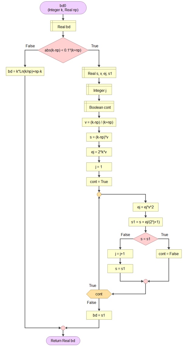
Loader's Algorithm
For large values of n, the calculations can take quite long, even for computers. Loader (2002) has derived an algorithm to make this easier. It is shown in figure 4, 5 and 6 as a flowchart.
Figure 4
Loader Algorithm part 1 of 3

Figure 5
Loader Algorithm part 2 of 3

Figure 6
Loader Algorithm part 3 of 3
With large sample sizes the binomial distribution will take quite some time to calculate. Thanks to computers this of course speeds up, but even for a computer this can become a challenge. If you keep on increasing n, the shape of the pmf starts to look like a bell shape, as illustrated in figure 7.
Figure 7
Binomial Distribution Increasing n Example

As it turns out, if n is large enough, the binomial distribution can be approximated by a normal distribution, which would save time in calculations. Note that if n is large, and p is small, then the binomial distribution could also be approximated with a Poisson distribution
Distributions
![]()

Google adds