
Distributions
Bivariate (Standard) Normal Distribution
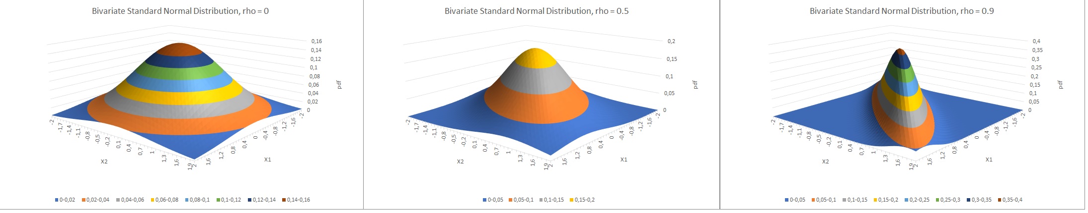
As the name implies a bivariate (standard) normal distribution, is what you get when you combine two (standard) normal distributions. Various definitions exist (see StatisticsHowTo.com for a few examples), but most often it is simply given by it's formula for the probability mass:
\( bsnpmf\left(x, y, \rho\right) = \frac{1}{2\times\pi} \times e^{-\frac{x^2 - 2\times\rho\times x\times y + y^2}{2\times\left(1 - \rho^2\right)}} \)
In this formula, \(\rho\) is the correlation between \(x\) and \(y\).
Figure 1 shows three visualisations of the bsnpmf for rho = 0, 0.5 and 0.9
Figure 1.
Bivariate Standard Normal Distribution examples.
SOCR has a nice website where you can play with various settings and see the visual result.
The bigger problem is calculating the volume under the area to get the cumulative density function. It would mean to solve the double integral:
\( bsncdf\left(x, y, \rho\right) = \int_{-\infty}^{x}\int_{-\infty}^{y}\frac{1}{2\times\pi} \times e^{-\frac{x^2 - 2\times\rho\times x\times y + y^2}{2\times\left(1 - \rho^2\right)}} \)
Many different algorithms are available for this, for example Owen (1956), Johnson and Kotz (1972), Donnelly (1973), Drezner (1978), Divgi (1979), Mee and Owen (1983), Baughman (1988), Moskowitz and Tsai (1989), Drezner and Wesolowsky (1990), Cox and Wermuth (1991), Albers and Kallenberg (1994), Lin (1995), West (2005), Meyer (2013), Vasicek (2015), Tsay and Ke (2021), and many more.
Owen used an additional function T, for which he made some large tables to look up the values, others have made algorithms to approximate these values, for example Cooper (1968, 1969), Borth (1973), Young and Minder (1974), Daley (1974), Wijsman (1996), and Patefield and Tandy (2000) (see Genz and Bretz (2009) for some overview and even more versions).
I've made myself an adoptation of the Tsay-Ke algorithm, by converting it to standard normal distribution, instead of the erf function they use. The math proof for this can be found here.
I also adopted the adaptation from Nikoloulopoulos from Johnson and Krotz algorithm to allow to specify how many terms you want to use for the precision. The math for this can be found here.
Use some software (easy)
Excel
Excel file: DI - Bivariate (Standard) Normal.xlsm
Excel unfortunately doesn't have a function so the file contains user-defined functions of the various algorithms. Alternatively Hull made a file available that has a function that uses Drezner's algorithm.
Flowgorithm
Owen
Owen's approach for the Bivariate Normal is shown in Figure 2.
Figure 2.
Bivariate Standard Normal Distribution - Owen.
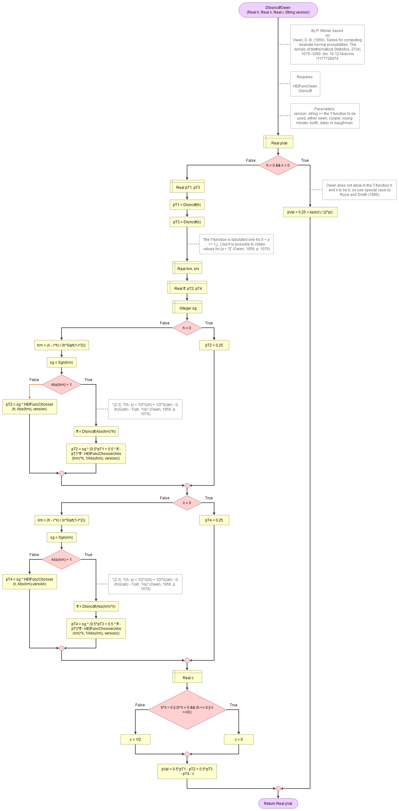
Flowgorithm: FL-DI-BivariateNormal-Owen.fprg
Various authors have suggested alternatives for the T-function used in Owen's approach. They are included in the flowgorithm file. The flow charts are shown below.
Owen T-function
Figure 3.
Bivariate Standard Normal Distribution - Owen's T-function.

Cooper T-function
Figure 4.
Bivariate Standard Normal Distribution - Cooper's T-function.

Borth T-function
Figure 5.
Bivariate Standard Normal Distribution - Borth's T-function.

Young and Minder T-function
Figure 6.
Bivariate Standard Normal Distribution - Young and Minder's T-function.

Daley T-function
Figure 7.
Bivariate Standard Normal Distribution - Daley's T-function.

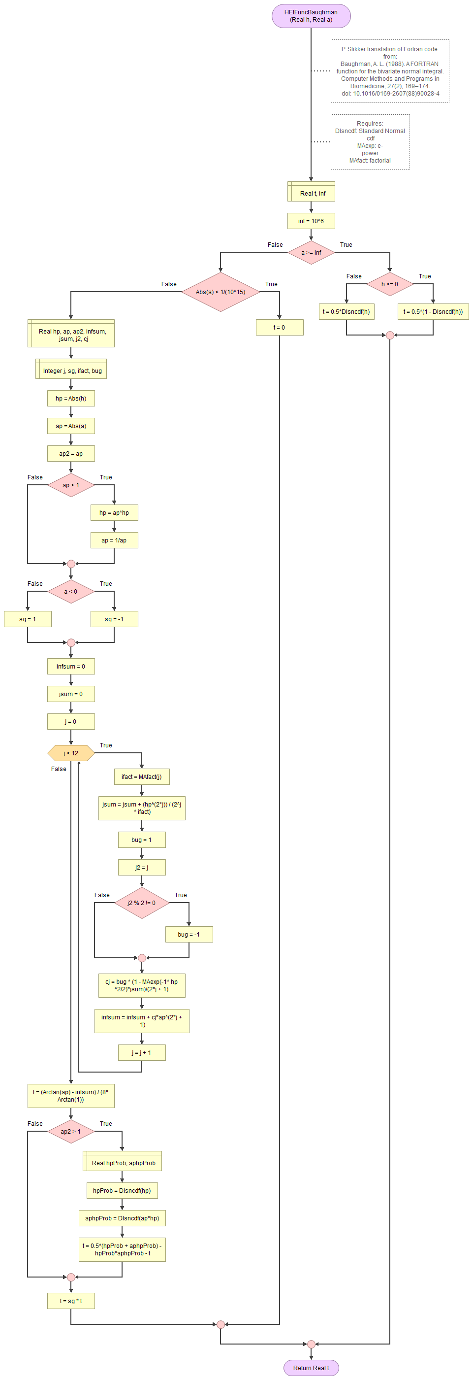
Baughman T-function
Figure 8.
Bivariate Standard Normal Distribution - Baughman's T-function.
Johnson and Kotz
Figure 1.
Bivariate Standard Normal Distribution - Johnson and Kotz.
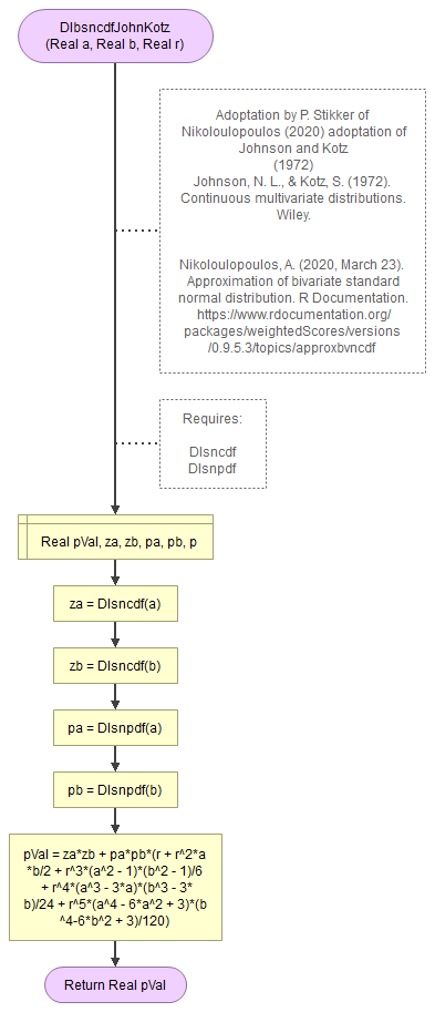
Flowgorithm: FL-DI-BivariateNormal-JohnsonKotz.fprg
Donnelly
Figure 1.
Bivariate Standard Normal Distribution - Donnelly.
Flowgorithm: FL-DI-BivariateNormal-Donnelly.fprg
Drezner
Figure 1.
Bivariate Standard Normal Distribution - Drezner.

Figure 2.
Drezner's helper function f.

Flowgorithm: FL-DI-BivariateNormal-Drezner.fprg
Mee and Owen
Figure 1.
Bivariate Standard Normal Distribution - Mee and Owen.

Flowgorithm: FL-DI-BivariateNormal-MeeOwen.fprg
Baughman
Figure 1.
Bivariate Standard Normal Distribution - Baughman.

Flowgorithm: FL-DI-BivariateNormal-Baughman.fprg
Drezner and Wesolowsky
Figure 1.
Bivariate Standard Normal Distribution - Drezner and Wesolowsky.
Flowgorithm: FL-DI-BivariateNormal-DreznerWesolowsky.fprg
Cox and Wermuth
Figure 1.
Bivariate Standard Normal Distribution - Cox and Wermuth.
Flowgorithm: FL-DI-BivariateNormal-CoxWermuth.fprg
Lin
Figure 1.
Bivariate Standard Normal Distribution - Lin.

Figure 2.
Lin's helper function for L.
Flowgorithm: FL-DI-BivariateNormal-Lin.fprg
West
Figure 1.
Bivariate Standard Normal Distribution - West.

Flowgorithm: FL-DI-BivariateNormal-West.fprg
Meyer
Figure 1.
Bivariate Standard Normal Distribution - Meyer.

Figure 2.
Meyer's helper function 1.

Figure 3.
Meyer's helper function 2.

Flowgorithm: FL-DI-BivariateNormal-Meyer.fprg
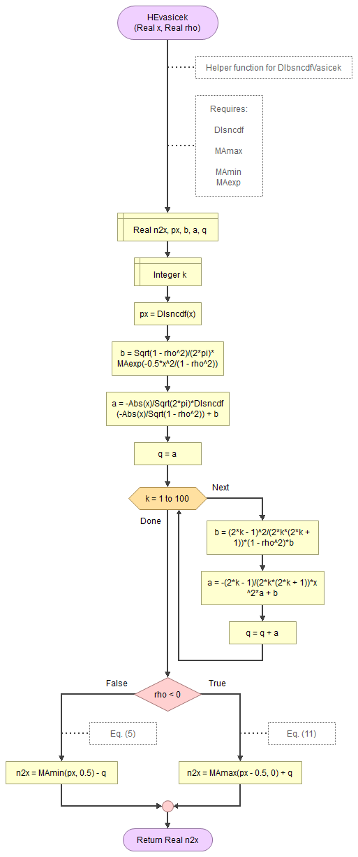
Vasicek
Figure 1.
Bivariate Standard Normal Distribution - Vasicek.

Figure 2.
Vasicek helper function.
Flowgorithm: FL-DI-BivariateNormal-Vasicek.fprg
Tsay and Ke
Figure 1.
Bivariate Standard Normal Distribution - Tsay and Ke.

Flowgorithm: FL-DI-BivariateNormal-TsayKe.fprg
Python
video to be uploaded
Jupyter Notebook: DI - Bivariate Normal.ipynb
Python itself does not have a bivariate normal distribution, but the scipy library has a general 'multivariate_normal' function.
R
R script: DI - Bivariate Normal.R
R itself doesn't have a bivariate normal distribution, but the libraries 'fMultivar' and 'VGAM' each have a function
SPSS
In SPSS, if you have one field with the \(x\) value, one with \(y\), and one with \(\rho\), you can use 'Transform - Compute variable'. Give the new variable a name (e.g. 'bsncdf'), and in the 'Function group' section select 'CDF & Noncentral CDF'. Then double click on the 'Cdf.Bvnor' function. Replace the question marks with your fields for \(x\), \(y\), and \(\rho\), and click on OK
Use the formulas (hard core)
The formula's for Owen and T-functions adaptations by Borth, and Daley can be found below, as well as for Johnson and Kotz, Drezner, Mee and Owen, Lin, Vasicek, and Tsay and Ke. Many others provided Fortran or C++ code. From those the code can be found in the flowgorithm section.
Owen (1956)
One of the earliest and often referenced algorithms is from Owen. In essence his approach is based on:
\(\Phi_2\left(x_1, x_2, \rho\right) = \frac{1}{2}\left(\Phi\left(x_1\right) + \Phi\left(x_2\right)\right) - T\left(x_1, \mu_{x_1}\right)- T\left(x_2, \mu_{x_2}\right) -c\)
In this formula \(\Phi\) is the standard normal distribution, and:
\(c = \begin{cases} 0 & \text{ if } x_1\times x_2 \gt 0 \text{ or } \left(x_1\times x_2 = 0 \text{ and } x_1+x_2 \ge 0\right) \\ \frac{1}{2} & \text{otherwise} \end{cases}\)
\(\mu_{x_1} = \frac{x_2-\rho\times x_1}{x_1\times\sqrt{1-\rho^2}}\)
\(\mu_{x_2} = \frac{x_1-\rho\times x_2}{x_2\times\sqrt{1-\rho^2}}\)
The big problem is that \(T\left(a, b\right)\) function. Owens states that this should only be used for cases where \(a \gt 0 \text{ and } 0 \lt b \le 1\), but gives a few useful methods to switch in case this is not the case:
\(T\left(a, -b\right) = -T\left(a, b\right)\)
\(T\left(-a, b\right) = T\left(a, b\right)\)
And in case that \(b \le 1\):
\(T\left(a, b\right) = \frac{1}{2}\left(sncdf\left(a\right) + sncdf\left(a\times b\right)\right) - sncdf\left(a\right) \times sncdf\left(a\times b\right) - T\left(a\times b, \frac{1}{b}\right)\)
The \(T\) function is then defined as:
\(T\left(a, b\right) = \frac{\arctan\left(b\right)}{2\times\pi} - \frac{1}{2\times\pi} \times \sum_{j=0}^{\infty} c_j\times b^{2\times j + 1}\)
With:
\(c_j = \left(-1\right)^j \times\frac{1}{2\times j+1}\times\left(1 - e^{-\frac{1}{2}\times a^2}\times\sum_{i=0}^j\frac{a^{2\times i}}{2^i\times i!}\right)\)
A few other useful values:
\(T\left(a, 0\right) = 0\)
\(T\left(0, b\right) = \frac{\arctan\left(b\right)}{2\times\pi}\)
Note however that although for \(T\), both \(a\) and \(b\) can be 0, for \(\Phi_2\) the values \(x_1\) and \(x_2\) cannot, since this will cause a division by 0 in \(\mu_x\).
However, those will then be close to infinity and Owen defines:
\(T\left(a,\infty\right) = \begin{cases} \frac{1}{2}\times\left(1-sncdf\left(a\right)\right) & \text{ if } a\ge 0 \\ \frac{1}{2}\times sncdf\left(a\right) & \text{ if } a\le 0 \end{cases}\)
Another special case of interest is:
\(\Phi_2\left(0, 0, \rho\right) = \frac{1}{4} + \frac{\arcsin\left(\rho\right)}{2\times\pi}\)
Other's have proposed different approaches for the T-function. The formula's from Borth and Daley are shown in the sections below, the algorithm from Cooper (1968), Young and Minder (1974) and Baughman (1988) can be found as a flowgorithm in the 'easy' section. Wijsman (1996) and Patefield and Tandy (2000) also made a T-function, but I haven't seen those.
T-function by Borth (1973)
Borth's adaptation of the T-function is:
\(T\left(h, a\right) = \frac{\sum_{k=0}^m C_{2\times k}\times I_{2\times k}\times\left(\frac{h}{\sqrt{2}}\right)^{-\left(2\times k +1\right)}}{2\times\pi\times e^{\frac{1}{2}\times h^2}}\)
With:
\(w = \frac{h\times a}{\sqrt{2}}\)
\(I_{2\times k} = \frac{1}{2}\times\left(\left(2\times k - 1\right)\times I_{2\times k - 2} - w^{2\times k - 1}\times e^{-w^2}\right)\)
\(I_0 = \sqrt{\pi}\times\left(\Phi\left(w\times\sqrt{2}\right) - \frac{1}{2}\right)\)
For the approximation Borth provides a table for the \(C_{2\times k}\) values. It is based on the coefficients of the Chebyshev polynomials. Borth gives the following table for this:
| k | \(C_{2\times k}\) |
|---|---|
0 |
0.9999936 |
1 |
-0.9992989 |
2 |
0.9872976 |
3 |
-0.9109973 |
4 |
0.6829098 |
5 |
-0.3360210 |
6 |
0.07612251 |
T-function by Daley (1974)
Daley rewrote the T function to:
\(T\left(x, y\right) = \frac{\arctan\left(y\right)}{2\times\pi\times e^{\frac{1}{2}\times x^2}}\times\left(1+\sum_{j=1}^{\infty}\frac{x^{2\times j}}{2^j\times j!} \times\left(1 - \frac{y}{\arctan\left(y\right)}\times\sum_{i=0}^{j-1}\frac{\left(-y^2\right)^i}{2\times i+1}\right)\right)\)
Johnson and Kotz (1972)
The R functionn 'approxbvncdf' in the 'weightedScores' library from Nikoloulopoulos (2020) is according to the info the method from Johnson and Kotz (1972).
\(\Phi_2(x,y,\rho) =\Phi(x)\times\Phi(y) + \phi(x)\times\phi(y)\times\sum_{j=1}^\infty \rho^j\times \psi_j(x)\times \psi_j(y)/j!\)
With:
\(\psi_j(z) = (-1)^{j-1}\times \frac{d^{j-1} \phi(z)}{dz^{j-1}}\)
To calculate the derivatives I made an iterative function (details):
\(\phi^x\left(z\right) = \left(-1\right)^x\times g_x \phi\left(z\right)\)
where \(\phi^x\left(z\right)\) is the \(x\)th derivative of \(\phi\left(z\right)\), and:
\(g_x = z^x + c_1\times z^{x-2} + c_2\times z^{x-4} + \dots\)
\(g_{x+1} = z^{x+1} + \left(c_1+x\right)\times z^{x-1} + \left(c_2 + c_1\times\left(x - 2\right)\right)\times z^{x-3} + \dots\)
The coefficients in general are then:
\(c_{x-1} = c_{c-2} + c_x\times\left(x-1\right)\)
Drezner (1978)
Drezner (1978) uses a Gauss quadrature and writes:
\(\Phi_2\left(x, y, \rho\right) = \frac{\sqrt{1 -\rho^2}}{\pi}\times\sum_{i,j=1}^y A_i\times A_j\times f\left(q_i, q_j\right)\)
Where:
\(f\left(q, r\right) = e^{x_1\left(2\times q-x_1\right) + y_1\times\left(2\times r-y_1\right) + 2\times\rho\times\left(2\times q-x_1\right)\times\left(2\times r-y_1\right)}\)
\(x_1 = \frac{x}{\sqrt{2\times\left(1 - \rho^2\right)}}\)
\(y_1 = \frac{y}{\sqrt{2\times\left(1 - \rho^2\right)}}\)
The values for \(A_i\) and \(q_i\) in the \(f\) function are from Steen, Byrne and Gelbard (1969).
However, this only works if \(x, y, \rho \le 0\), but using formulas from Johnson and Kotz other scenarios can be rewritten to:
If \(x\times y\times\rho \le0\) do:
\(\Phi_2\left(x, y, \rho\right) = \begin{cases} \Phi_2\left(x, y, \rho\right) & , x\le 0, y\le 0, \rho \le 0 \\ \Phi\left(x\right) - \Phi_2\left(x, -y, -\rho\right) & , x\le 0, y\ge 0, \rho \ge 0 \\ \Phi\left(y\right) - \Phi_2\left(-x, y, -\rho\right) & , x\ge 0, y\le 0, \rho \ge 0 \\ \Phi\left(y\right) + \Phi\left(y\right) - 1 + \Phi_2\left(-x, -y, \rho\right) & , x\ge 0, y\ge 0, \rho \le 0\end{cases}\)
Else (Owen, 1957, p. 11):
\(\Phi_2\left(x, y, \rho\right) = \Phi_2\left(x, 0, \rho\left(x,y\right)\right) + \Phi_2\left(y, 0, \rho\left(y,x\right)\right) - c\)
with:
\(\rho\left(a, b\right) = \frac{\left(\rho\times a - b\right)\times \text{Sign}\left(a\right)}{\sqrt{a^2-2\times\rho\times a\times b + b^2}}\)
\(c = \frac{1-\text{Sign}\left(x\right)\times\text{Sign}\left(y\right)}{4}\)
\(\text{Sign}\left(i\right) = \begin{cases} 1 & ,i\ge 0 \\ -1 & i \lt 0 \end{cases}\)
Note that originally Drezner has for \(c\) a '1 + ...' in the denominator, but I think this should be '1 - ...'
Mee and Owen (1983)
In this approach an approximation is used:
\(\Phi_2\left(x, y,\rho\right) \approx \Phi\left(x\right)\times\Phi\left(\frac{y - \mu}{\sigma}\right)\)
With:
\(\mu = -\frac{\rho\times\phi\left(x\right)}{\Phi\left(x\right)}\)
\(s = \sqrt{1 + \rho\times x\times\mu - \mu^2}\)
If \(\left|x\right| \lt \left|y\right|\) swop \(x\) and \(y\) and then use:
\(\Phi_2\left(x, y,\rho\right) = \begin{cases} \Phi_2\left(x, y,\rho\right) & ,\text{if } x \le 0 \\ \Phi\left(y\right) - \Phi_2\left(-x, y,-\rho\right) & ,\text{if } x \gt 0 \end{cases}\)
Lin (1995)
A relative simple algorithm was made by Lin, although not very accurate compared to some of the others. Lin gives a function for the upper-tail using:
\(L_2\left(x, 0, \rho\right) = \frac{1}{\sqrt{8\times a}}\times e^{\frac{b^2}{4\times a}}\times Q\left(\sqrt{2\times a}\times\left(x + \frac{b}{2\times a}\right)\right)\)
Where \(Q\) is the complement function of the normal cdf, ie:
\(Q\left(z\right) = 1 - \phi\left(z\right)\)
Further defined are:
\(a = 0.5 + 0.416\times\frac{\rho^2}{1-\rho^2}\)
\(b = 0.717\times\frac{-\rho}{\sqrt{1-\rho^2}}\)
This is enough Zelen and Severo (1960) already showed:
\(L_2\left(x, y, \rho\right) = L_2\left(x, 0, \rho\left(x,y\right)\right) + L_2\left(y, 0, \rho\left(y,x\right)\right) - \frac{1}{2}\times c\)
\(\rho\left(i, j\right) = \frac{\left(\rho\times i - k\right)\times \text{Sign}\left(i\right)}{\sqrt{i^2 - 2\times\rho\times i\times j + j^2}}\)
\(\text{Sign}\left(i\right) = \begin{cases} 1 & \text{,if } i \ge 0 \\ -1 & \text{,if } i \lt 0\end{cases}\)
\(c = \begin{cases} 0 & \text{,if } x\times y \ge 0 \\ 1 & \text{,if } x\times y \lt 0\end{cases}\)
We can convert this to the lower tail using:
\(\Phi_2\left(x, y, \rho\right) = L_2\left(x, y, \rho\right) - 1 + \Phi\left(x\right)+ \Phi\left(y\right)\)
Similar as with Drezner we can also make use of:
\(\Phi_2\left(x, y, \rho\right) = \begin{cases} \Phi\left(x\right) - \Phi_2\left(x, -y, -\rho\right) & , x\le 0, y\ge 0 \\ \Phi\left(y\right) - \Phi_2\left(-x, y, -\rho\right) & , x\ge 0, y\le 0 \\ \end{cases}\)
Vasicek (2015)
Vasivic works using the identity:
\(\Phi_2\left(x, y, \rho\right) = \Phi_2\left(x, 0, \rho\left(x, y\right)\right) + \Phi_2\left(y, 0, \rho\left(y, x\right)\right) - c\)
Where:
\(\rho\left(i, j\right) = \frac{\left(\rho\times i - k\right)\times \text{Sign}\left(i\right)}{\sqrt{i^2 - 2\times\rho\times i\times j + j^2}}\)
\(\text{Sign}\left(i\right) = \begin{cases} 1 & \text{,if } i \ge 0 \\ -1 & \text{,if } i \lt 0\end{cases}\)
\(c = \begin{cases} 0 &\text{ if } x\times y \gt 0 \\ \frac{1}{2} &\text{ if } x\times y \lt 0 \end{cases}\)
Vasivic then defines:
\(\Phi_2\left(x, 0, \rho\right) = \begin{cases} \min\left(\Phi\left(x\right), \frac{1}{2}\right) - Q &\text{ if } \rho \gt 0 \\ \max\left(\Phi\left(x\right) - \frac{1}{2}, 0\right) + Q &\text{ if } \rho \lt 0 \end{cases}\)
The problem is calculating \(Q\) which is defined as:
\(Q = \sum_{k=0}^{\infty} A_k\)
To calculate \(A_k\) an iterative process is proposed:
\(B_0 = \frac{\sqrt{1 - \rho^2}}{2\times\pi} \times e^{-\frac{1}{2}\times\frac{x^2}{1-\rho^2}}\)
\(A_0 = -\frac{\left|x\right|}{2\times\pi}\times \Phi\left(-\frac{\left|x\right|}{\sqrt{1-\rho^2}}\right) + B_0\)
And then for the next values:
\(B_k = \frac{\left(2\times k - 1\right)^2}{2\times k\times\left(2\times k + 1\right)}\times\left(1 - \rho^2\right)\times B_{k-1}\)
\(A_k = \frac{2\times k - 1}{2\times k\times\left(2\times k + 1\right)}\times x^2 \times A_{k-1} + B_{k}\)
Tsay and Ke (2021)
Tsay and Ke (2021) propose a set of 5 equations depending on different situations, using the error function (erf). I adapted this to use the normal distribution instead (details) .
\(\Phi_2\left(x, y, rho\right) = \begin{cases} \Phi\left(y\right) + \Phi\left(\frac{b}{a}\right) - 1 + f_1\times\left(f_3\times\left(1 - \Phi\left(v_5\right)\right) - f_4\times\left(\Phi\left(v_7\right) + \Phi\left(v_6\right) - 1\right)\right) & ,\text{if } a\gt 0 \text{ and } a\times y + b \ge 0 \\ f_1\times f_3\times\Phi\left(v_8\right) & ,\text{if } a\gt 0 \text{ and } a\times y + b \lt 0 \\ \Phi\left(x\right)\times\Phi\left(y\right) & ,\text{if } a = 0 \\ \Phi\left(y\right) - f_1\times f_2\times\Phi\left(v_7\right) & ,\text{if } a\lt 0 \text{ and } a\times y + b \ge 0 \\ 1 - \Phi\left(\frac{y}{x}\right) + f_1\times\left(f_3\times\left(\Phi\left(v_8\right) + \Phi\left(v_5\right) - 1\right) - f_4\times\left(1 - \Phi\left(v_6\right)\right)\right) & ,\text{if } a\lt 0 \text{ and } a\times y + b \lt 0 \end{cases}\)
With:
\(a = \frac{-\rho}{\sqrt{1-\rho^2}}, b = \frac{x}{\sqrt{1-\rho^2}}\)
\(c_1 = -1.09500814703333\)
\(c_2 = -0.75651138383854\)
\(f_1 = \frac{1}{2\times\sqrt{1-a^2\times c_2}}\)
\(f_2 = e^{f_1^2\times\left(a^2\times c_1^2 + 2\times b^2\times c_2\right)}\)
\(f_3 = f_2\times e^{-f_1^2\times 2\times\sqrt{2}\times b\times c_1}\)
\(f_4 = \frac{1}{f_3}\)
\(v_5 = \frac{f_1}{a}\times\left(2\times b - \sqrt{2}\times a^2\times c_1\right)\)
\(v_5 = \frac{f_1}{a}\times\left(2\times b + \sqrt{2}\times a^2\times c_1\right)\)
\(v_7 = f_1\times\left(2\times y - 2\times a^2\times c_2\times y - 2\times a\times b\times c_2 - \sqrt{2}\times a\times c_1\right)\)
\(v_8 = f_1\times\left(2\times y - 2\times a^2\times c_2\times y - 2\times a\times b\times c_2 + \sqrt{2}\times a\times c_1\right)\)
Distributions
![]()

Google adds