
Distributions
(Standard) Normal Distribution
The APA dictionary of Statistics and Research Methods defines the normal distribution as "a theoretical distribution in which values pile up in the center at the mean and fall off into tails at either end" (Zedeck, 2014, p. 238). It often appears in statistics and looks like a bell, but should follow a specific formula (see formula's for the scary looking formula).
Note that not every bell-shape distribution is a normal distribution. The formula requires a mean and standard deviation. However, any normal distribution can be converted to a standard normal distribution.
The standard normal distribution is a specific normal distribution, for which the population mean is fixed as zero, and the sample variance as one. So by substracting the mean and dividing the result by the standard deviation, any normal distribution gets converted to a standard normal distribution. By subtracting the mean and dividing by the standard deviation you get something called a z-score. It tells how many standard deviations something was away from the mean. It gives an indication on how rare a particular score is.
Four examples are shown of a normal distribution in figure 1.
Figure 1Examples of Normal Distribution

Note that the peak of the curve is always at the mean, and the higher the standard deviation, the 'flatter' the bell looks.
As with any continuous distribution it is very important to remember that we are usually only interested in the areas under the curve, since those give us the probability
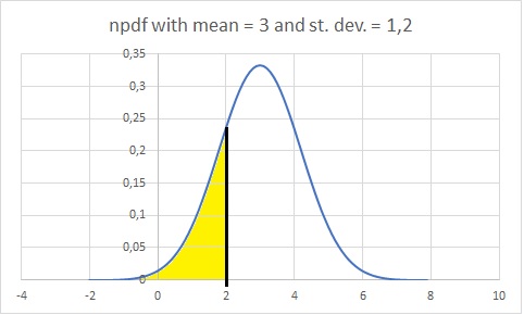
For example the probability of a z-value less than 2, in a normal distribution with a mean of 3 and a standard deviation of 1.2 would be the area highlighted in yellow in figure 2.
Figure 2Example of Area under Normal Distribution
Now calculating this area can be tricky business depending on how easy you want to make it on yourself
Use some software (easy)
Excel
In short: The function NORM.S.DIST with the z-value and 'cumulative' set to TRUE, will give the cdf, while if it is set to FALSE the pdf is returned.
Excel file: DI - Normal.xlsm
Flowgorithm
The rar file contains 60+ approximations for the normal distributions. These are discussed in the 'Do the math' section.
Rar file with 62 Flowgorithm files: DI-Normal.rar
Python
In short: After installing scipy, the norm module can be loaded using 'from scipy.stats import norm'. The cdf is then obtained using norm.cdf(z), the complement using norm.sf(z), the pdf using norm.pdf(z), and the inverse using norm.ppf(prob).
Python's statistics also has a normal library. First load using 'from statistics import NormalDist'. The cdf can then be obtained using NormalDist().cdf(z), the pdf using NormalDist().pdf(z), and the inverse using NormalDist().inv_cdf(prob)
Jupyter Notebook: DI - Normal.ipynb
R
The cdf is obtained using pnorm(z), the complement using pnorm(z, lower.tail = FALSE), the pdf using dnorm(z), and the inverse using qnorm(prob).
Video to be upladed
R script: to be uploaded
SPSS
Use tables (old school)
Before computers we often made use of tables, like the one shown in figure 3.
Figure 2Cumulative Standard Normal Distribution Table

To illustrate how to use this, let's imagine we had a z-value of -0.53, and want to know the probability of having a z-value of -0.53 or less (assuming a normal distribution)
First you notice all the values are positive, so how can we find -0.53? Well, the standard normal distribution is symmetrical around the center which is at 0. The area under the curve for -0.53 or less, is the same as the area under the curve for 0.53 or more.
Great, so we just look up 0.53? Nope, because now we need 0.53 or more, while the table will only show us 0.53 or less. Luckily the total area under the curve should be 1, so what we could do is determine the probability for a z-value of 0.53 or less, and then subtract this from 1.
To find this probability we look for the integer and first decimal in the first column, in this example 0.5. Then look in that row at the column which has the second decimal, in the example the 0.03. This is highlighted in figure 3
Figure 3Cumulative Standard Normal Distribution Table Example

We find the value of 0.70194. That is the probability for a z-value of 0.53 or less. After we subtract this from 1, we get 1 - 0.70194 = 0.29806, as the probability of a z-value of -0.53 or less.
You might wonder if we should have excluded 0.53 itself, but for a continuous distribution the probability for exactly a z-value of 0.53 or any z-value will be next to 0 (1 / infinity), so no we don't need to worry about that.
With statistical tests we often need the probability of an event or even more extreme. This means an event as likely or even less likely than a z-value of -0.53. This is therefor also a z-value of 0.53 or more. Since the distribution is symmetrical we can simply double the one-sided -0.53 probability we found and get 2 times 0.29806 = 0.59612.
Do the math (hard core)
\( npdf\left(x, \mu, \sigma\right) = \frac{1}{\sigma\times\sqrt{2\times\pi}}\times e^{-\frac{1}{2}\times\left(\frac{x-\mu}{\sigma}\right)^2} \)
If the mean \( \mu \) is equal to 0, and the standard deviation \(\sigma\) equal to 1 we can simplify this a little
\( snpdf\left(z\right) = \phi\left(z\right) = \frac{1}{1\times\sqrt{2\times\pi}}\times e^{-\frac{1}{2}\times\left(\frac{z-0}{1}\right)^2} \)
\( = \frac{1}{\sqrt{2\times\pi}}\times e^{-\frac{1}{2}\times z^2} \)
Which is the formula for the standard normal distribution probability density function.
To calculate the areas underneath the curve for less than z, we can use the integral
\( sncdf\left(z\right) = \Phi\left(z\right) = \int_{x=|Z|}^{\infty}\left(\frac{1}{\sqrt{2\times\pi}}\times e^{-\frac{z^2}{2}}\right) \)
Use Bars to approximate
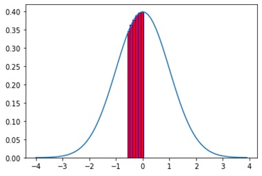
One way to calculate this integral is to split the area in small rectangles, and use the npdf to calculate the height
Let's say we wanted to calculate the probability of a z-value of -0.53 or less. Now since the normal distribution is symmetrical, we know that the probability of a z-value of 0 or less is 0.5. If we subtract the probability of a z-value between -0.53 and 0 from this, we should get our desired result
We start with placing a very thin vertical bar at -0.53 with a width of only 0.03, and the height equal to npdf(-0.53), then a small vertical bar from -0.50 to -0.40 (a widht of 0.1) with a height of npdf(-0.50), a bar from -0.40 to -0.30 with height npdf(-0.40), a bar from -0.30 to -0.20 with height npdf(-0.30), a bar from -0.20 to -0.10 with height npdf(-0.20), and finally one from -0.10 to 0 with height npdf(-0.10). This is illustrated in figure 4.
Figure 3Normal Integral Calculation
So the first bar will have a height of:
\( snpdf\left(-0.53\right) = \frac{1}{\sqrt{2\times\pi}}\times e^{-\frac{1}{2}\times \left(-0.53\right)^2} \approx 0.3467 \)
Since the width of this first bar is 0.03, the area of this bar will be 0.03 × 0.3467 \(\approx\) 0.0104
For the second bar we get as height:
\( snpdf\left(-0.5\right) = \frac{1}{\sqrt{2\times\pi}}\times e^{-\frac{1}{2}\times \left(-0.5\right)^2} \approx 0.3521\)
Which has a width of 0.10, so an area of 0.10 × 0.3521 \(\approx\) 0.0352
The calculations for the other bars:
\( 0.10\times snpdf\left(-0.4\right) = \frac{1}{\sqrt{2\times\pi}}\times e^{-\frac{1}{2}\times \left(-0.4\right)^2} \approx 0.10\times 0.3683 \approx 0.0368\)
\( 0.10\times snpdf\left(-0.3\right) = \frac{1}{\sqrt{2\times\pi}}\times e^{-\frac{1}{2}\times \left(-0.3\right)^2} \approx 0.10\times 0.3814 \approx 0.0381\)
\( 0.10\times snpdf\left(-0.2\right) = \frac{1}{\sqrt{2\times\pi}}\times e^{-\frac{1}{2}\times \left(-0.2\right)^2} \approx 0.10\times 0.3910 \approx 0.0391\)
\( 0.10\times snpdf\left(-0.1\right) = \frac{1}{\sqrt{2\times\pi}}\times e^{-\frac{1}{2}\times \left(-0.1\right)^2} \approx 0.10\times 0.3970 \approx 0.0397\)
Now we add them all up to get: 0.0104 + 0.0352 + 0.0368 + 0.0381 + 0.0391 + 0.0397 = 0.1993. So this is the very rough approximate probability of a z-value between -0.53 and 0. But wait...we needed to subtract this from 0.5, which gives: 0.5 - 0.1993 = 0.3007. So this is our estimate for the probability of a z-value of -0.53 or less.
The actual probability would actually be closer to 0.2981 but this was just as an illustration. You can get better approximations by creating more bars with thinner widths, and/or use a trapezium at the end, but hope this example was good enough to get the idea.
Numerical approximation
There are also many different numerical approximations. I tried grouping them a bit in different categories.
Note that some approximations were more to try to get a 'simple' equation, some more on an 'accurate', some on a time efficient, and some to allow for an easy inverse cdf to be derived. Because of this, a newer approximation is not necesairily 'better'.
A small note on the original sources. Some original sources will have referenced Abromowitz and Stegun, but this refers to a book from them, and the chapter in there with the approximations for the normal cdf is written by Zelen and Severo, so I listed them.
For the numeric and computer algorithms, the table below gives an overview of the different versions I managed to find. If you know of another, please let me know:
| Author | Year | Category | Comment |
|---|---|---|---|
| Abderrahmane and Boukhetala | 2016 | Mill's ratio/Error | |
| Abernathy | 1988 | Sums | |
| Adams | 1969 | Computer | |
| Aludaat and Alodat | 2008 | Error | |
| Badhe | 1976 | Sets | |
| Bagby | 1995 | Other | |
| Bowling et al. | 2009 | logistic | two variations |
| Bryc | 2002 | Mill's ratio | three variations |
| Bunday, Bokhari, and Khan | 1997 | Computer | |
| Burr | 1967 | Other | two variations |
| Cadwell | 1951 | Error | two variations |
| Choudhury | 2014 | Mill's ratio | |
| Choudhury, Ray, and Sarkar | 2007 | Sets | |
| Choudhury and Roy | 2009 | Sets | |
| Cody | 1969 | Sets | |
| Cody | 1993 | Computer | |
| Cooper | 1968 | Computer | |
| Crawford and Techo | 1962 | Computer | with remarks from Hill and Joyce (1967) |
| Cyvin | 1964 | Computer | with remarks from Hill and Joyce (1967) |
| Derenzo | 1977 | Sets | |
| Divgi | 1979 | Mill's ratio | |
| Dridi | 2003 | Sets | |
| Eidous and Al-Salman | 2016 | Error | |
| Hamaker | 1978 | Error | |
| Hart | 1957 | Mill's ratio | |
| Hart | 1966 | Mill's ratio | |
| Hastings | 1955 | Mill's ratio/Sums | six variations |
| Hawkes | 1982 | Sets | |
| Hill | 1973 | Computer | |
| Hill and Joyce | 1967 | Computer | with remarks from Bergson (1968), Adams (1969), and Holmgren (1970) |
| Ibbetson | 1963 | Computer | |
| Kerridge and Cook | 1976 | Sums | |
| Kiani et al. | 2008 | Sets | |
| Lew | 1981 | Sets | two variations |
| Lin | 1988 | Error | |
| Lin | 1989 | Other | |
| Lin | 1990 | Logistic | |
| Marsaglia | 2004 | Computer | |
| Matić, Radoičić, and Stefanica | 2018 | Error/Sets | two variations |
| Milton and Hotchkiss | 1969 | Computer | |
| Moran | 1980 | Sums | two variations |
| Norton | 1989 | Sums | two variations |
| Page | 1977 | Trigonometry | |
| Patry and Keller | 1964 | Other | |
| Polya | 1949 | Error | same as Williams |
| Raab and Green | 1961 | Trigonometry | Formula found in Page |
| Schucany and Gray | 1968 | Mill's ratio | for z&2 only |
| Shah | 1985 | Sets | |
| Shchigolev | 2020 | Other | |
| Shore | 2005 | Other | three variations |
| Smits | 1981 | Computer | |
| Soranzo and Epure | 2014 | Other | |
| Strecok | 1968 | Other | |
| Thacher | 1963 | Computer | Large z only, with remarks from Hill and Joyce (1967) |
| Tocher | 1963 | Trigonometry | |
| Vazquez et al. | 2012 | Trigonometry | |
| Vedder | 1993 | logistic/trigonometry | |
| Waissi and Rossin | 1996 | Logistic | |
| West | 2005 | Computer | |
| Williams | 1946 | Error | same as Polya |
| Winitzki | 2008 | Error | |
| Yerukala and Boiroju | 2015 | Trigonometry/Mill's Ratio | three variations |
| Yerukala, Boiroju, and Reddy | 2011 | Trigonometry | |
| Yun | 2009 | Trigonometry | two variations |
| Zelen and Severo | 1970 | Mill's ratio/Sums | four variations |
Single equations - Using Error Function
The approximations in this section, all have the format of:
\(\Phi\left(z\right) \approx \frac{1}{2}\times\left(1 + \sqrt{1 - \alpha}\right)\)
They come from the relation between the sncdf and the error function. The error function is defined as:
\( \text{Erf}\left(x\right) = \frac{2}{\sqrt{\pi}}\int_{i=0}^x e^{-i^2} \)
This can then be converted to the sncdf by using:
\( \Phi\left(z\right) = \frac{1 + \text{Erf}\left(\frac{z}{\sqrt{2}}\right)}{2}\)
One that is often referenced is Polya (1949), although this article was from a conference that was held in 1946. The same approximation was also published by Williams (1946) who gets far less often referenced. The approximation:
\(\Phi\left(z\right) \approx \frac{1}{2}\times\left(1 + \sqrt{1 - e^{-\frac{2\times z^2}{\pi}}}\right)\)
Cadwell (1951) improved on this using:
\(\Phi\left(z\right) \approx \frac{1}{2}\times\left(1 + \sqrt{1 - e^{-\frac{2\times z^2}{\pi}+ \frac{2\times\left(\pi - 3\right)\times z^4}{3\times\pi^2}} }\right)\)
Cadwell also noted that since the above formula was not asymptotically correct another adjustment for Polya/Williams:
\(\Phi\left(z\right) \approx \frac{1}{2}\times\left(1 + \sqrt{1 - e^{-\frac{2\times z^2}{\pi}} - 0.0005\times z^6 + 0.00002\times z^8}\right)\)
Strecok (1968) uses the error function as well, but with a summation and sinus operator. See the Single 'simple' equations - With Sums section for this approach
Hamaker (1978) continued on the work from Page (1977) and Zelen and Severo, but then actually came up with a formula very similar to the ones above.
\(\Phi\left(z\right) \approx \frac{1}{2}\times\left(1 + \text{sign}\left(z\right)\times\sqrt{1 - e^{-\left(0.806\times \left|z\right|\times\left(1 -\times0.018\times\left|z\right|\right)\right)^2}}\right)\)
Lin (1988) further improved on Hamaker's equation:
\(\Phi\left(z\right) \approx \frac{1}{2}\times\left(1 + \sqrt{1 - e^{-\left(\frac{z}{1.237+0.0249\times z}\right)^2}}\right)\)
Aludaat and Alodat (2008) looked at Polya, Chokri, Bailey and Johnson, but found that the equations were either too complicated or that the inverse was complicated or impossible. They proposed:
\(\Phi\left(z\right) \approx \frac{1}{2}\times\left(1 + \sqrt{1 - e^{-\sqrt{\frac{\pi}{8}}\times z^2}}\right)\)
Winitzki (2008) proposes:
\(\Phi\left(z\right) \approx \frac{1}{2}\times\left(1 + \sqrt{1 - e^{-\frac{z^2}{2}\times\frac{\frac{8}{\pi}+0.147\times z^2}{2+0.147\times z^2}}}\right)\)
Eidous and Al-Salman (2016) noted that Aludaat and Alodat's improvement on Polya was not fully proven to be an improvement as an upper bound and improved on it themselves by adjusting it to:
\(\Phi\left(z\right) \approx \frac{1}{2}\times\left(1 + \sqrt{1 - e^{-\frac{5}{8}\times z^2}}\right)\)
Note that they also shown that this is an improvement over Bowling et. al () and Lin (), which will be discussed later. The maximum absolute error was stated to be 0.00180786.
Abderrahmane and Boukhetala (2016) also looked at Aludaat and Alodat's improvement of Polya and improved on it themselves to:
\(\Phi\left(z\right) \approx \frac{1}{2}\times\left(1 + \sqrt{1 - e^{-0.62306179\times z^2}}\right)\)
They don't seem to have considered Eidos and Al-Salman's version, however they state that their maximum absolute error is 0.001622801925711, slightly less than the other. Note that they also made another approximation based on a different one, to be discussed later below.
Matić, Radoičić, and Stefanica (2018) compared many different approximations, and gave the following of their own:
\(\Phi\left(z\right) \approx \frac{1}{2}\times\left(1 + \sqrt{1-e^{-\frac{2\times z^2}{\pi}\times\left(1+\sum_{k=1}^5 a_{2\times k}\times z^{2\times k}\right)}}\right)\)
Single equations - Using Logistic Approximation
The approximations in this section all have a format of:
\(\Phi\left(z\right) \approx \frac{1}{1+e^{\alpha}}\)
Lin (1990) uses a logistic approximation on the previous section, specifically from Hamaker and Lin (1988). The approximation proposed is:
\(\Phi\left(z\right) \approx \frac{1}{1+e^{-\frac{4.2\times\pi\times z}{9-z}}}\)
Vedder (1993) improved on this with:
\(\Phi\left(z\right) \approx \frac{1}{1+e^{-\sqrt{\frac{8}{\pi}}\times z - \frac{4-\pi}{3\times\pi}\times\sqrt{\frac{2}{\pi}}\times z^3}}\)
Waissi and Rossin (1996) gave a three parameter approximation:
\(\Phi\left(z\right) \approx \frac{1}{1+e^{-\sqrt{\pi}\times\left(-0.0004406\times z^5+0.0418198\times z^3+0.9\times z\right)}}\)
Bowling et al. (2009) continued the work and gave two approximations. One with one parameter, and one with two. Bowling does not reference Waissi and Rossin nor Vedder.
\(\Phi\left(z\right) \approx \frac{1}{1+e^{-1.702\times z}}\)
\(\Phi\left(z\right) \approx \frac{1}{1+e^{-\left(0.07056\times z^3+1.5976\times z\right)}}\)
Single equations - Using Mill's Ratio
Mill's ratio is another function that is approximated from which the normal cdf can be approximated. These have the general form of:
\(\Phi\left(z\right) \approx 1-\phi\left(z\right)\times f\left(z\right)\)
Mill's ratio for the normal distribution can be defined as:
\(R\left(z\right) =e^{-z^2}\times\int_{i=z}^\infty e^{-\frac{i^2}{2}}\)
This can then be converted to the sncdf by using:
\( \Phi\left(z\right) = 1 -R\left(z\right)\times\phi\left(z\right)\)
Hastings (1955) looks at the error function but this can be converted to the Mill's ratio. Hasting proposes to use:
\(\text{erf}\left(x\right) \approx 1 - \frac{2}{\sqrt{\pi}}\times e^{-x^2}\times\sum_{i=1}^k a_i\times t^i\)
This can be re-written to the form of:
\(\Phi\left(z\right) \approx 1-\phi\left(z\right)\times \sqrt{2} \times \sum_{i=1}^k a_i\times t^i\)
With:
\(t = \frac{1}{p\times x}\)
\(x = \frac{z}{\sqrt{2}}\)
And Hastings gives three different sets for \(p\) and \(a_i\):
Version 1 - Sheet 43
\(p = 0.47047, a_{1\dots 3} = \left\{0.3084284,-0.0849713,0.6627698\right\}\)
Version 2 - Sheet 44
\(p = 0.381965, a_{1\dots 4} = \left\{0.12771538,0.54107939,-0.53859539,0.75602755\right\}\)
Version 3 - Sheet 45
\(p = 0.3275911, a_{1\dots 4} = \left\{0.225836846,-0.252128668,1.25969513,-1.287822453,0.94064607\right\}\)
Note: Version 1 and 3 can be found as well in Abramowitz and Stegun’s book, in chapter 7 written by Gautschi (1970) as Algorithm 7.1.25 and Algorithm 7.1.26 resp.. The values for a_i are multiplied by 2/√π, and the equation adjusted accordingly
Hart (1957) uses the Mill's Ratio, and proposed:
\(\Phi\left(z\right) \approx 1-\frac{\phi\left(z\right)}{z+0.8\times e^{-0.4\times z}}\)
Hart (1966) proposed:
\(\Phi\left(z\right) \approx 1 - \frac{\phi\left(z\right)}{z}\times\left(1 - \frac{\frac{\sqrt{1+c\times z^2}}{1+b\times z^2}}{a\times z+\sqrt{a^2\times z^2+e^{-\frac{z^2}{2}}}\times\frac{\sqrt{1+c\times z^2}}{1+b\times z^2}}\right)\)
with:
\(a = \sqrt{\frac{\pi}{2}} \)
\(b = \frac{1+\sqrt{1-2\times\pi^2+6\times\pi}}{2\times\pi} \)
\(c = 2\times\pi\times b^2\)
Schucany and Gray (1968) improved on Hart (1966), and proposed for z>2:
\(\Phi\left(z\right) \approx 1 - \frac{z\times\phi\left(z\right)}{z^2+2}\times\frac{z^6+6\times z^4-14\times z^2 - 28}{z^6+5\times z^4-20\times z^2 - 4}\)
Zelen and Severo (1970) for version 1 and 2:
\(\Phi\left(z\right) \approx 1 - \phi\left(z\right)\times\sum_{i=1}^k a_i\times\left(\frac{1}{1+p\times z}\right)^i\)
With for version 1:
\( p=0.33267, a_{k=3,1\dots3}\left\{0.4361836,-0.1201676,0.937298\right\} \)
and for version 2:
\( p=0.2316419, a_{k=5,1\dots5}\left\{0.319381530,-0.356563782,1.781477937,-1.821255978,1.330274429\right\} \)
Note that version 1 is also sometimes referenced as from Texas Instruments (1980, as cited in McConnell (1981))
Divgi (1979) also use the Mill's ratio with a summation over 11 values:
\(\Phi\left(z\right) \approx 1 - \phi\left(z\right)\times\sum_{i=0}^n a_i\times z^i\)
With:
\( a_{i=0\dots 10}\left\{1.253313402, -0.9999673043,0.6262972801, -0.3316218430, 0.1522723563, -5.982834993\times 10^{-2}, 1.915649350\times 10^{-2}, -4.644960579\times 10^{-3}, 7.771088713\times 10^{-4}, -7.830823677\times 10^{-5}, 3.534244658\times 10^{-6}\right\} \)
Bryc (2002) gave a more precise version of this as:
\(\Phi\left(z\right) \approx 1-\frac{\left(4-\pi\right)\times z+\sqrt{2\times\pi}\times\left(\pi-2\right)}{\left(4-\pi\right)\times z^2 + 2\times\left(\pi-2\right)+\sqrt{2\times\pi}\times z} \times\phi\left(z\right)\)
which got approximated to:
\(\Phi\left(z\right) \approx 1-\frac{z+0.333}{\sqrt{2\times\pi}\times z^2+7.32\times z + 6.666} \times e^{-\frac{z^2}{2}}\)
The author also proposed a second iteration for Mill's ratio and approximated that with:
\(\Phi\left(z\right) \approx 1-\frac{z^2+5.575192695\times z+12.77436324}{\sqrt{2\times\pi}\times z^3+14.38718147\times z^2 + 31.53531977\times z +25.54872648} \times e^{-\frac{z^2}{2}}\)
Choudhury (2014) compared various approximations, including Bryc's (but doesn't reference Hart) and derived:
\(\Phi\left(z\right) \approx 1-\frac{\phi\left(z\right)}{0.226+0.64\times z+0.33\times\sqrt{z^2+3}}\)
Yerukala and Boiroju (2015) second approximation, does not fit the general format of this section, but is a combination of Hart and Byrc's approximations:
\(\Phi\left(z\right) \approx 0.268\times\Phi_{Hart}\left(z\right) + 0.732\times\Phi_{Byrc}\left(z\right)\)
Yerukala and Boiroju (2015) third approximation is a modification of Choudhury (2014) (see error function):
\(\Phi\left(z\right) \approx 1 - \phi\left(z\right)\times\frac{\sqrt{2\times\pi}}{\frac{44}{79}+\frac{8}{5}\times z+\frac{5}{6}\times\sqrt{z^2+3}}\)
Abderrahmane and Boukhetala (2016) besides an approximation based on the error function, also gave an improvement on Hart's approximation as:
\(\Phi\left(z\right) \approx 1-\frac{\phi\left(z\right)}{z+0.79758\times e^{-0.4446\times z}}\)
Single equations - Using trigonometry
A few approximation use trigonometry, with almost all using the hyperbolic tangent function (tanh).
The tanh approximations use:
\(\frac{e^{2\times\alpha}}{1+e^{2\times\alpha}} = \frac{1}{2}\times\left(1+\text{tanh}\left(\alpha\right)\right)\)
Raab and Green (1961) proposed:
\(\Phi\left(z\right) \approx = 1 - \frac{1+\cos\left(z\right)}{\pi}\times\frac{\pi - z -\sin\left(z\right)}{2\times\pi}\)
This approximation seems to be the worst of all of them, but is interestingly the only one with sinus and cosine.
Thocher (1963) proposed (re-written in tanh form):
\(\Phi\left(z\right) \approx \frac{1}{2}\times\left(1+\text{tanh}\left(\sqrt{\frac{2}{\pi}}\times z\right)\right)\)
Strecok (1968) uses the error function as well, but with a summation and sinus operator. See the Single 'simple' equations - With Sums section for this approach
Page (1977) improved on this with:
\(\Phi\left(z\right) \approx \frac{1}{2}\times\left(1+\text{tanh}\left(\sqrt{\frac{2}{\pi}}\times z\times\left(1+0.044715\times z^2\right)\right)\right)\)
Moran (1980) improved on the work from Strecok, also with a summation and sinus operator. See the Single 'simple' equations - With Sums section for this approach
Vedder (1993) also gave a tanh version of the approximation shown in the logistic section:
\(\Phi\left(z\right) \approx \frac{1}{2}\times\left(1+\text{tanh}\left(\frac{1}{2}\times z\times\left(\sqrt{\frac{8}{\pi}}+\frac{4-\pi}{3\times\pi}\times\sqrt{\frac{2}{\pi}}\times z^2\right)\right)\right)\)
Yun (2009) had the following approximation:
\(\Phi\left(z\right) \approx \frac{1}{2}\times\left(1 + \tanh\left(\frac{18.445}{20}\times\left(\frac{1}{\left(1-\frac{z}{\sqrt{\frac{\pi}{2}}\times18.445}\right)^{10}} - \frac{1}{\left(1+\frac{z}{\sqrt{\frac{\pi}{2}}\times18.445}\right)^{10}}\right)\right)\right)\)
Yun (2009) also simplified the approximation using the inverse of tanh
\(\Phi\left(z\right) \approx \frac{1}{2}\times\left(1+\text{tanh}\left( 2.5673\times\text{atanh}\left(\frac{z}{\sqrt{\frac{\pi}{2}}\times2.5673}\right)\right)\right)\)
Yerukala et al. (2011) used a neural network approach and found:
\(\Phi\left(z\right) \approx 0.5 - 1.136\times\text{tanh}\left(-0.2695\times z\right) + 2.47\times\text{tanh}\left(0.5416\times z\right) - 3.013\times\text{tanh}\left(0.4134\times z\right)\)
They tested this against Polya, Lin, Aludaat and Alodat, and Bowling, and found this outperforms those. The max absolute error was 0.0013 for z-values between 0 and 3.
Vazquez et al. (2012) derived an approximation which then got converted into fractions, and then to exponential:
\(\Phi\left(z\right) \approx \frac{1}{2} \times \left(1 + \text{tanh}\left(\frac{39\times z}{2\times\sqrt{2\times\pi}} - \frac{111}{2} \times \text{atan}\left(\frac{35\times z}{111\times\sqrt{2\times\pi}}\right)\right)\right)\)
\(\Phi\left(z\right) \approx \frac{1}{2} \times \left(1 + \text{tanh}\left(\frac{179\times z}{23} - \frac{111}{2} \times \text{atan}\left(\frac{37\times z}{294}\right)\right)\right)\)
\(\Phi\left(z\right) \approx \frac{1}{1+e^{-\frac{358\times z}{23}+111\times\text{tanh}\left(\frac{37\times z}{294}\right)}}\)
Yerukala and Boiroju (2015) propose:
\(\Phi\left(z\right) \approx \frac{1}{1+e^{-0.125-3.611\times\tanh\left(0.043+0.2624\times z\right)+4.658\times\tanh\left(-1.687-0.519\times z\right)-4.982\times\tanh\left(-1.654+0.5044\times z\right)}} \)
Single equations - With Sums
The approximations in this section all use a summation.
Hastings (1955) proposed
\(\Phi\left(z\right) \approx 1 - \frac{1}{2\times\left(1+\sum_{i=1}^k a_i\times\left(\frac{z}{\sqrt{2}}\right)^i\right)^{2^k -z}}\)
Hastings gave three different suggestions for \(a_i\):
\(a_{k=4, 1\dots4} = \left\{0.278393,0.230389,0.000972,0.078108\right\}\)
\(a_{k=5, 1\dots5} = \left\{0.14112821,0.08864027,0.02743349,0.00039446,0.00328975\right\}\)
\(a_{k=6, 1\dots6} = \left\{0.0705230784,0.0422820123,0.0092705272,0.0001520143,0.0002765672,0.000430638\right\}\)
Strecok (1968) uses the sinus to approximate the error function with:
\(\text{erf}\left(x\right) \approx \frac{2}{\pi}\times\left(\frac{x}{5}+\sum_{n=1}^{37} \frac{1}{n}\times e^{-\left(\frac{n}{5}\right)^2}\times\sin\left(\frac{2\times n\times x}{5}\right)\right)\)
Zelen and Severo (1970) for version 3 and 4:
\(\Phi\left(z\right) \approx 1 - \frac{1}{2\times\left(1+\sum_{i=1}^k a_i\times z^i\right)^{2^{k-2}}}\)
With for version 3:
\( a_{k=3,1\dots3}\left\{0.196854,0.115194,0.000344,0.019527\right\} \)
and for version 4:
\( a_{k=6,1\dots6}\left\{0.0498673470,0.0211410061,0.0032776263,0.000380036,0.0000488906,0.0000053830\right\} \)
Kerridge and Cook (1976) use the following infinite series:
\(\Phi\left(z\right) \approx 1 - \frac{1}{2} + \phi\left(z\right)\times z\times\sum_{i=0}^{\infty}\frac{a_{2\times i}}{2\times i + 1}\)
With the recursive function:
\( a_i = \frac{z^2}{4}\times\frac{a_i-a_{i-1}}{n+1} \)
\( a_0 = 1, a_1 = \frac{z^2}{4} \)
Moran (1980) continues on the work from Strecock (1968) and suggests two similar approximations. Version 1:
\(\Phi\left(z\right) \approx \frac{1}{2} + \frac{1}{\pi}\times\left(\frac{z}{3\times\sqrt{2}} + \sum_{n-1}^{\infty} \frac{e^{\frac{-n^2}{9}}}{n}\times\sin\left(\frac{n\times z\times\sqrt{2}}{3}\right)\right)\)
and version 2:
\(\Phi\left(z\right) \approx \frac{1}{2} + \frac{1}{\pi}\times\left(\sum_{n-1}^{\infty} \frac{e^{\frac{\left(n+\frac{1}{2}\right)^2}{9}}}{n+\frac{1}{2}}\times\sin\left(\frac{\left(n+\frac{1}{2}\right)\times z\times\sqrt{2}}{3}\right)\right)\)
Moran mentions that version 1 when n = 12 will be accurate to nine decimal places while z ≤ 7, and for version 2 when n = 7.
Abernathy (1988) uses a series expansion of \(e^x\) very similar to Mill's ratio:
\(\Phi\left(z\right) \approx \frac{1}{2} + \frac{1}{\sqrt{2\times\pi}}\times\sum_{n=0}^\infty \frac{\left(-1\right)^n\times z^{2\times n+1}}{2^n\times n!\times\left(2\times n + 1\right)}\)
Single equations - Other
Patry and Keller (1964) proposed (using the error function):
\(\Phi\left(z\right) \approx 1 - \frac{e^{-\frac{z^2}{2}}\times t}{2\times 1.77245385\times\left(\frac{z}{\sqrt{2}}\times t+1\right)}\)
with:
\(t = 1.77245385+\frac{z}{\sqrt{2}}\times\left(2-q\right) \)
\(q = \frac{0.858407657+\frac{z}{\sqrt{2}}\times\left(0.307818193+\frac{z}{\sqrt{2}}\times\left(0.0638323891-\frac{z}{\sqrt{2}}\times0.000182405075\right)\right)}{1+\frac{z}{\sqrt{2}}\times\left(0.650974265+\frac{z}{\sqrt{2}}\times\left(0.229484819+\frac{z}{\sqrt{2}}\times 0.0340301823\right)\right)}\)
Burr (1967) proposed:
\(\Phi_{\text{Burr}}\left(z\right) \approx 1 - \left(1 + \left(0.644693 + 0.161984\times z\right)^{4.874}\right)^{-6.158}\)
Version 2 was a modification using:
\(\Phi\left(z\right) \approx \frac{\Phi_{\text{Burr}}\left(z\right)+1-\Phi_{\text{Burr}}\left(-z\right)}{2}\)
Lin (1989) proposed:
\(\Phi\left(z\right) \approx 1 - \frac{e^{-0.717\times z - 0.416\times z^2}}{2}\)
This came from using an ordinary least square to find the optimal solution for values using:
\( 1 - \Phi\left(z\right) \approx \frac{e^{b\times z + a\times z^2}}{2} \)
Bagby (1995) proposed:
\(\Phi\left(z\right) \approx \frac{1}{2}\times\left(1+\sqrt{1-\frac{1}{30}\times\left(7\times e^{-\frac{z^2}{2}}+16\times e^{-z^2\times\left(2-\sqrt{2}\right)}+ \left(7+\frac{\pi}{4}\times z^2\right)\times e^{-z^2}\right)}\right)\)
Note that this resembles a lot format of the error function based equations.
Shore (2005) created three variations using the RMM error distribution. Version 1 looks as follows:
\(\Phi\left(z\right) \approx 1 - e^{-\ln\left(2\right)\times e^{b\times\left(e^{c\times z}-1\right) + d\times z}}\)
With:
\(b=-1.81280,c=-0.472245,d=0.294549\)
For version 2 and 3 the following is used:
\(\Phi\left(z\right) \approx \frac{1+g\left(-z\right)-g\left(z\right)}{2}\)
With for version 2:
\(g\left(z\right) = e^{-\ln\left(2\right)\times e^{b\times\left(e^{a+c\times z}-1\right)+d\times z}}\)
\(a=0.072880383,b=-2.36699428,c=-0.40639929,d=0.19417768\)
and for version 3:
\(g\left(z\right) = e^{-\ln\left(2\right)\times e^{\frac{a\times b}{c}\times\left(\left(1+b\times z\right)^{\frac{c}{b}}-1\right)+d\times z}}\)
\(a=-6.37309208,b=-0.11105481,c=-0.61228883,d=0.44334159\)
Soranzo and Epure (2014) gave a very different formula as an approximation, compared to the others:
\(\Phi\left(z\right) \approx 2^{-22^{1-41^{z/10}}}\)
Shchigolev (2020) used a Variational Iteration Method to derive the following approximation:
\(\Phi\left(z\right) \approx \frac{1}{2} + \frac{1}{\sqrt{2}}\times\left(7-\left(7+3\times\sqrt{2}\times z+\frac{5}{4}\times z^2 + \frac{\sqrt{2}}{4}\times z^3 + \frac{z^4}{8}\right)\times e^{-\frac{z}{\sqrt{2}}}\right)\)
Set of Equations
Cody (1969) gives the following set of equations for the error function:
\(\text{erf}\left(z\right) \approx \begin{cases} x\times R\left(x^2\right) & \text{if } \left|x\right|≤0.5 \\ 1 - e^{-x^2}\times R\left(x\right) & \text{if } 0.46875≤x≤4 \\ 1 - \frac{e^{-x^2}}{x}\times\left(\frac{1}{\sqrt{\pi}} + \frac{1}{x^2}\times R\left(\frac{1}{x^2}\right)\right) & \text{if } x≥4 \end{cases}\)
With:
\(R\left(x\right) = \frac{\sum_{i=0}^n p_i\times x^i}{\sum_{i=0}^n q_i\times x^i}\)
The values for \(p_i\) and \(q_i\) are given by Cody in various tables.
Badhe (1976) continued on the results from Patry and Keller (1964) and gave the following three approximations:
For \(z≥2\):
\(\Phi\left(z\right) \approx 1 - \phi\left(z\right) \times \frac{1}{z}\times\left(1-\frac{1}{y}\times\left(1+\frac{1}{y}\times\left(7+1/y\times\left(55+\frac{1}{y}\times\left(445+37450\times \frac{q}{y}\right)\right)\right)\right)\right)\)
With:
\(q=1+\frac{8.5}{z^2-\frac{0.4284639753}{z^2}+1.240964109}\)
\(y = z^2+10\)
For \(z<2\):
\(\Phi\left(z\right) \approx \frac{1}{2}+z\times\left(a_1+y\times\left(a_2+y\times\left(a_3+y\times\left(a_4+y\times\left(a_5+y\times\left(a_6+y\times\left(a_7+a_8\times y\right)\right)\right)\right)\right)\right)\right)\)
With:
\(y=\frac{z^2}{32}\)
\(a_{i=1\dots 8} = \left\{0.3989422784,-2.127690079,10.2125662121,-38.8830314909,120.2836370787,-303.2973153419,575.073131917,-603.9068092058\right\}\)
Derenzo (1977) approximation:
\(\Phi\left(z\right) \approx \begin{cases} 1-\frac{1}{2}\times e^{-\frac{\left(83\times z+351\right)\times z + 562}{\frac{703}{z}+165}} & \text{ if } z<5.5 \\ 1 - \frac{\sqrt{\frac{2}{\pi}}}{2\times z}\times e^{-\frac{z^2}{2}-\frac{0.94}{z^2}}& \text{ if } z≥5.5 \end{cases}\)
Lew (1981) gives two approximation sets:
version 1:
\(\Phi\left(z\right) \approx \begin{cases} \frac{1}{2}+\frac{z-\frac{1}{7}\times z^3}{\sqrt{2\times\pi}} & \text{ if } 0 ≤z≤1 \\ 1 - \frac{\left(1+z\right)\times\phi\left(z\right)}{z^2+z+1} & \text{ if } z>1 \end{cases}\)
version 2:
\(\Phi\left(z\right) \approx \begin{cases} \frac{1}{2}+\frac{2}{5}\times z & \text{ if } 0 ≤z≤\frac{1}{2} \\ 1 - \frac{\left(1+z\right)\times\phi\left(z\right)}{z^2+z+1} & \text{ if } z>\frac{1}{2} \end{cases}\)
Hawkes (1982):
\(\Phi\left(z\right) \approx \begin{cases} \frac{1}{2}\times\left(1 + \sqrt{1-e^{-2\times\frac{t^2}{\pi}}}\right) & \text{ if } 0 ≤z≤2.2 \\ 1 - \frac{\left(1.184+z\right)\times\phi\left(z\right)}{z^2+1.176\times z+1.209} & \text{ if } z>2.2 \end{cases}\)
With:
\( t=z-\frac{7.5166\times z^3}{10^3}+\frac{3.1737\times z^5}{10^4} - \frac{2.9657\times z^7}{10^6}\)
Shah (1985) gives perhaps a not so accurate, but the perhaps the most simple approximation:
\(\Phi\left(z\right) \approx \begin{cases} \frac{1}{2}+\frac{z\times\left(4.4-z\right)}{10} & \text{ if } 0 ≤z≤2.2 \\ 0.99 & \text{ if } 2.2<z<2.6 \\ 1 & \text{ if } z≥2.6 \end{cases}\)
Norton (1989) builds further on Shah's set, and gives two sets:
version 1:
\(\Phi\left(z\right) \approx \begin{cases} 1-\frac{1}{2}\times e^{-\frac{z^2+z}{2}} & \text{ if } 0 ≤z≤2.6 \\ 1-\frac{\phi\left(z\right)}{z} & \text{ if } z>2.6 \end{cases}\)
version 2:
\(\Phi\left(z\right) \approx \begin{cases} 1-\frac{1}{2}\times e^{-\frac{z^2+1.2\times z^0.8}{2}} & \text{ if } 0 ≤z≤2.7 \\ 1-\frac{\phi\left(z\right)}{z} & \text{ if } z>2.7 \end{cases}\)
Dridi (2003) gives an approximation set for the error function, based on rational fractions. It's a modification of Cody's algorithm
\(\text{erf}\left(x\right) \approx \begin{cases} x\times R_1\left(x^2\right) & \text{ if } 0 ≤x≤1.5 \\ 1 - e^{-x^2}\times\left(\frac{1}{2}\times R_1\left(x^4\right)+\frac{1}{5}\times R_2\left(x^{-4}\right)+\frac{3}{10}\times R_3\left(\frac{1}{x^{-4}}\right)\right) & \text{ if } 0.46875≤x≤4 \\ 1 - \frac{e^{-x^2}}{x}\times\left(\frac{1}{\sqrt{\pi}}+\frac{1}{x^2}\times R\left(\frac{1}{x^2}\right)\right) & \text{ if } x≥4 \end{cases}\)
With:
\(R_i\left(x\right) = \frac{\sum_{i=0}^n p_i\times x^i}{\sum_{i=0}^n q_i\times x^i}\)
The values for \(p_i\) and \(q_i\) are given by Cody in various tables or can be obtained from the example code provided by Dridi.
Choudhury, Ray, and Sarkar (2007):
If \(0 < z ≤ 0.7315 \text{ or } 2.2075 < z ≤ 2.7245 \text{ or } 3.056 < z≤4\):
\(\Phi\left(z\right) \approx 1-\frac{z^2+5.575192695\times z+12.77436324}{z^3\times\sqrt{2\times\pi}+14.38718147\times z^2 +31.53531977\times z+25.548726}\times e^{-\frac{z^2}{2}} \)
If \(0.7315 < z ≤ 1.726 \text{ or } 1.8135 < z ≤ 2.2075\):
\(\Phi\left(z\right) \approx 1-\left(0.4361836\times t-0.1201676\times t^2+0.937298\times t^3\right)\times\phi\left(z\right) \)
With \( t = \frac{1}{1+0.33267\times z} \)
If \(1.726 < z ≤ 1.8135 \text{ or } 2.7245 < z ≤ 3.056\):
\(\Phi\left(z\right) \approx \frac{1}{2}\times\left(1 + \sqrt{1 - \frac{1}{30}\times\left(7\times e^{-\frac{z^2}{2}}+16\times e^{-z^2\times\left(2-\sqrt{2}\right)} + \left(7+\frac{\pi\times z^2}{4}\right)\times e^{-z^2}\right)}\right) \)
Kiani, Panaretos, Psarakis, and Saleem (2008):
\( \Phi\left(z\right) \approx \frac{1}{2}\times\left(1-\text{sign}\left(-z\right)\times\sqrt{1-e^{-z^2\times w\left(z\right)}}\right) \)
If \(0 ≤ \left|z\right| < 1.05 \):
\( w\left(z\right) = -\frac{6.62}{10^6}\times\left|z\right|^5 +\frac{4.4166}{10^4}\times z^4 - \frac{1.31}{10^5}\times\left|z\right|^3 - \frac{94661}{9900000}\times z^2 - \frac{4.8}{10^7}\times\left|z\right| + \frac{7073553}{11111111}\)
If \(1.05 ≤ \left|z\right| < 2.29 \):
\( w\left(z\right) = -\frac{1.401663}{10^4}\times\left|z\right|^5 +\frac{1.150811}{10^3}\times z^4 - \frac{1.582555}{10^3}\times\left|z\right|^3 - \frac{7.76126}{10^3}\times z^2 - \frac{1.0608}{10^3}\times\left|z\right| + 0.6368751 \)
If \(2.29 ≤ \left|z\right| < 8 \):
\( w\left(z\right) = \frac{5.8716}{10^5}\times\left|z\right|^5 -\frac{1.221684}{10^3}\times z^4 + \frac{9.841663}{10^3}\times\left|z\right|^3 - \frac{3.55101}{10^2}\times z^2 + \frac{3.29203}{10^2}\times\left|z\right| + 0.62010268 \)
If \(8 ≤ \left|z\right| \):
\( w\left(z\right) = 0.5 \)
Choudhury and Roy (2009):
\(\text{erf}\left(x\right) \approx \begin{cases} \frac{1}{2} + \phi\left(z\right)\times g\left(z\right) & \text{ if } 0 <z<1.8735 \\ a+b\times z + c\times z^2 + \frac{1}{2} + \phi\left(z\right)\times g\left(z\right) & \text{ if } 1.8735≤z≤2.0885 \\ \alpha+\beta\times z + \gamma\times z^2 + 1 - \frac{1}{2}\times \phi\left(z\right)\times h\left(z\right) & \text{ if } 2.0885<z≤2.43 \\ 1 - \frac{1}{2}\times\phi\left(z\right)\times h\left(z\right) & \text{ if } 2.43 <z≤5.75 \\ 1 & \text{ if } z>5.75 \end{cases}\)
With:
\(g\left(z\right) = \frac{654729075\times z+45945900\times z^3+6486480\times z^5+154440\times z^7+4785\times z^9}{654729075-172297125\times z^2+20270250\times z^4-1351350\times z^6+51975\times z^8-945\times z^10} \)
\( a=-0.00007237,b=0.00007680,c=-0.00002041 \)
\( h\left(z\right) = \frac{2\times z^9+88\times z^7+1176\times z^5+5280\times z^3+5790\times z}{z^10+45\times z^8+630\times z^6+3150\times z^4+4725\times z^2+945} \)
\( \alpha=-0.00004861, \beta=0.00004021,\gamma=-0.00000833 \)
Computer Algorithms
The following computer algorithms were found in various sources:
- Crawford and Techo (1962) - Algorithm 123 (for the error function)
- Thacher (1963) - Algorithm 180 (for large values of z only) (for the error function)
- Remarks by Hill and Joyce (1967)
- Ibbetson (1963) - Algorithm 209
- Cyvin (1964) - Algorithm 226
- Remarks by Hill and Joyce (1967)
- Hill and Joyce (1967) - Algorithm 304
- Cooper (1968) - Algorithm AS 2
- Adams (1969) - Algorithm 39
- Milton and Hotchkiss (1969) - Fortran function CDFN
- Hill (1973) - Algorithm AS 66
- Smits (1981) - Fortran function ZPROB
- Cody (1993) - Algorithm 715
- Bunday-Bokhari-Khan (1997) - Pseudo code
- Marsaglia (2004) - C function Phi
- West (2004) - VBA function Cumnorm
Distributions
![]()

Google adds