
Analyse a Single Nominal Variable
The analysis of a single nominal variable can be done with the steps shown below. Click on each step to reveal how this step can be done.
Step 1: Impression
For a quick impression of a nominal variable, you can create a frequency table. The result will be something as shown in table 1.
| Frequency | Percent | Valid Percent | Cumulative Percent | ||
|---|---|---|---|---|---|
| Valid | Married | 972 |
49.2 |
50.1 |
50.1 |
| Widowed | 181 |
9.2 |
9.3 |
59.4 |
|
| Divorced | 314 |
15.9 |
16.2 |
75.6 |
|
| Separated | 79 |
4.0 |
4.1 |
79.6 |
|
| Never married | 395 |
20.0 |
20.4 |
100.0 |
|
| Subtotal | 1941 |
98.3 |
100.0 |
||
| Missing | No answer | 33 |
1.7 |
||
| Subtotal | 33 |
1.7 |
|||
| Total | 1974 |
100.0 |
Click here to see how to create a frequency table with Excel, Python, R, or SPSS.
with Python
Jupyter Notebook of video is available here.
with stikpetP library
without stikpetP library
with R (Studio)
with stikpetP library
Jupyter Notebook of video is available here.
without stikpetR library
R script of video is available here.
Datafile used in video: GSS2012-Adjusted.sav
with SPSS
There are a three different ways to create a frequency table with SPSS.
An SPSS workbook with instructions of the first two can be found here.
using Frequencies
watch the video below, or download the pdf instructions (via bitly, opens in new window/tab).
Datafile used in video: Holiday Fair.sav
using Custom Tables
watch the video below, or download the pdf instructions for versions before 24, or version 24 (via bitly, opens in new window/tab)
Datafile used in video: Holiday Fair.sav
using descriptive shortcut
watch the video below, or download the pdf instructions (via bitly, opens in new window/tab).
Datafile used in video: StudentStatistics.sav
See the explanation of frequency table for details on how to read this kind of table.
In the example we can see that Married has been chosen quite often compared to the others, and Separated the least. The table itself might not end up in the report, but gives a quick impression for yourself. Most would probably prefer a visualisation though.
Step 2: Visualisation
To visualise the results of a single nominal variable a simple bar-chart is often a good choice. An example is shown in Figure 1.
Figure 1
Results of marital status

Click here to see how to create a bar-chart
with Excel
Excel file from video VI - Bar Chart (Simple).xlsm.
with Python
Jupyter Notebook from video: VI - Bar Chart (Simple).ipynb.
Data file used: GSS2012a.csv.
with R (Studio)
R script from video VI - Bar Chart (Simple).R.
Data file used: GSS2012-Adjusted.sav.
with SPSS
There are a few different ways to obtain a (simple) bar-chart with SPSS. The end result for each will be the same.
using Chart builder
Watch the video below, or follow the instructions in this pdf (via bitly, opens in new window/tab).
Data file used: StudentStatistics.sav.
using Legacy dialogs
Watch the video below, or follow the instructions in this pdf (via bitly, opens in new window/tab).
Data file used: StudentStatistics.sav.
using Frequencies
Watch the video below, or follow the instructions in this pdf (via bitly, opens in new window/tab).
Data file used: StudentStatistics.sav.
using an existing table
Watch the video below, or follow the instructions in this pdf (via bitly, opens in new window/tab)
Data file used: StudentStatistics.sav.
When showing a bar-chart it is good to also talk a little bit about it. Usually the peak is mentioned (known as the mode) and perhaps a few of the very low ones. It always depends on the situation, but inform your reader what you notice from the graph or what you want to show.
In the report I recommend using a ‘Introduce – Show – Tell’ approach. Introduce the figure, then show the figure, then talk about what you notice. The example shows the same as we also saw from the frequency table; Married is chosen by far the most, and separated the least.
There are some alternatives for a bar-chart, these include pie-chart, (Cleveland) dotplot, and Pareto chart.
Step 3: Overall Test
The previous steps, gave an impression on the sample results, but are the results also significant? We can test if the percentages could be equal for all categories, in the population with a Pearson chi-square goodness-of-fit test.
Click here to see how to perform a Pearson chi-square goodness-of-fit test
with Excel
Excel file from video: TS - Pearson chi-square GoF.xlsm.
with Flowgorithm
A basic implementation for Pearson Chi-Square GoF test in the flowchart in figure 1
Figure 1
Flowgorithm for the Pearson Chi-Square GoF test
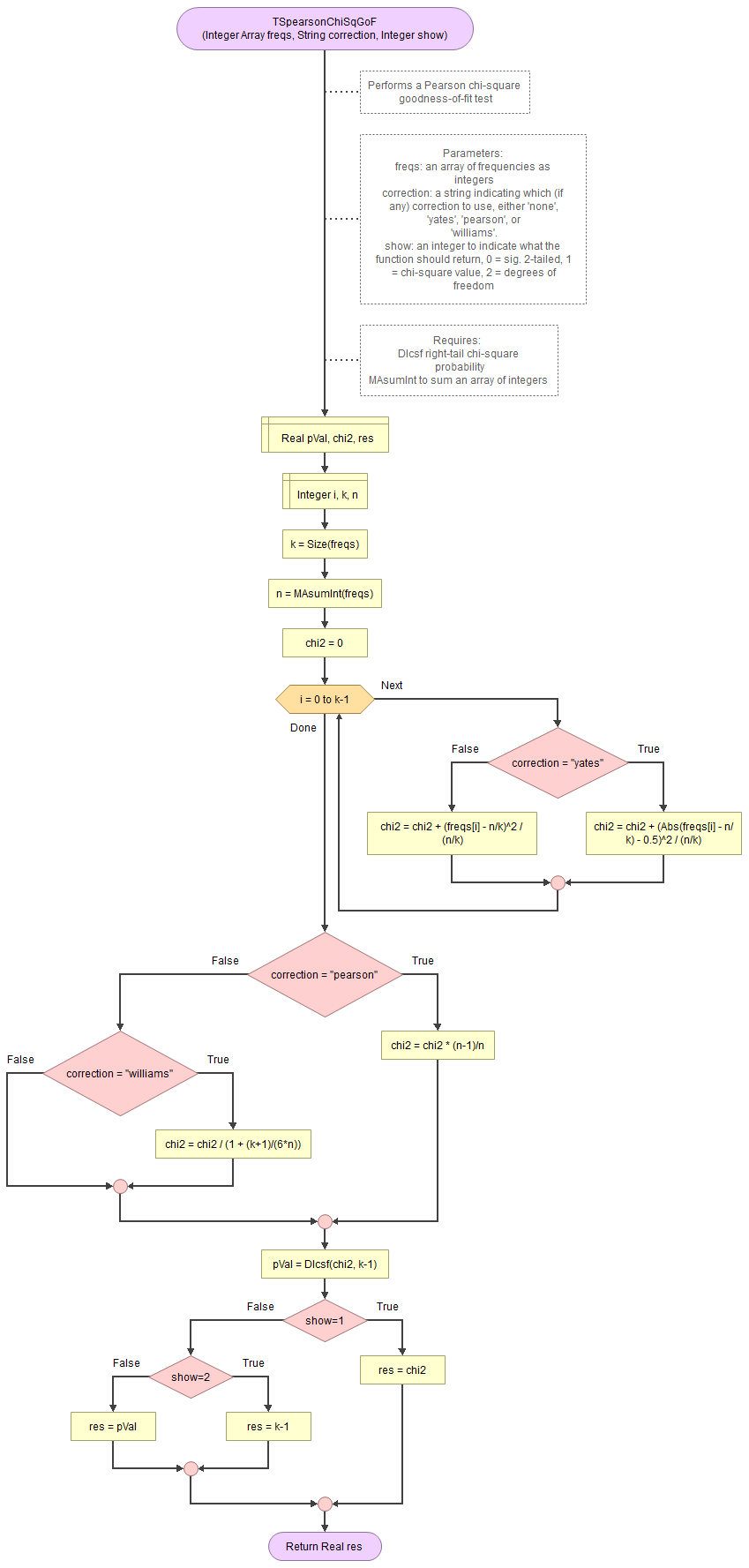
It takes as input an array of integers with the observed frequencies, a string to indicate which correction to use (either 'none', 'pearson', 'williams', or 'yates') and an integer for which output to show (0 = sig., 1=chi-square value, 2 = degrees of freedom).
It uses the function for the right-tail probabilities of the chi-square distribution and a small helper function to sum an array of integers.
Flowgorithm file: FL-TSpearsonChiSqGoF.fprg.
with Python
Jupyter Notebook from video: TS - Pearson chi-square GoF.ipynb.
Data file from video: GSS2012a.csv.
with R (Studio)
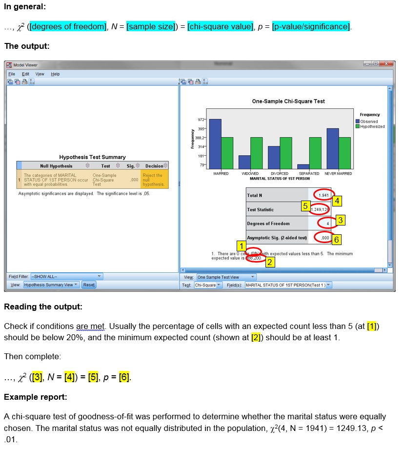
Click or hover over the thumbnail below to see where to look in the output.

R script from video: TS - Pearson chi-square GoF.R.
Data file from video: Pearson Chi-square independence.csv.
with SPSS
via One-sample
Click or hover over the thumbnail below to see where to look in the output.
Data file used in video: GSS2012-Adjusted.sav.
via Legacy dialogs
Click or hover over the thumbnail below to see where to look in the output.

Data file used in video: GSS2012-Adjusted.sav.
Manually (Formula and example)
The formula's
The Pearson chi-square goodness-of-fit test statistic (χ2):
\( \chi^{2}=\sum_{i=1}^{k}\frac{\left(O_{i}-E_{i}\right)^{2}}{E_{i}}\)
In this formula Oi is the observed count in category i, Ei is the expected count in category i, and k is the number of categories.
If the expected frequencies, are expected to be equal, then:
\(E_{i}=\frac{\sum_{j=1}^{k}O_{i}}{k}\)
The degrees of freedom is given by:
\(df=k-1\)
The probability of such a chi-square value or more extreme, can then be found using the chi-square distribution.
Example
We have the following observed frequencies of five categories:
\(O=\left(972,181,314,79,395\right)\)
Note that since there are five categories, we have k = 5. If the expected frequency for each category is expected to be equal we can use the formula to determine:
\(E_{i}=\frac{\sum_{j=1}^{k}O_{i}}{k}=\frac{\sum_{j=1}^{5}O_{i}}{5} =\frac{972+181+314+79+395}{5}\)
\(=\frac{1941}{5}=388\frac{1}{5}=388.2\)
Then we can determine the Pearson chi-square value:
\(\chi^{2}=\sum_{i=1}^{k}\frac{\left(O_{i}-E_{i}\right)^{2}}{E_{i}}=\sum_{i=1}^{5}\frac{\left(O_{i}-\frac{1941}{5}\right)^{2}}{\frac{1941}{5}}\)
\(=\frac{\left(972-\frac{1941}{5}\right)^{2}}{\frac{1941}{5}}+\frac{\left(181-\frac{1941}{5}\right)^{2}}{\frac{1941}{5}}+\frac{\left(314-\frac{1941}{5}\right)^{2}}{\frac{1941}{5}}+\frac{\left(79-\frac{1941}{5}\right)^{2}}{\frac{1941}{5}}+\frac{\left(395-\frac{1941}{5}\right)^{2}}{\frac{1941}{5}}\)
\(=\frac{\left(\frac{972\times5}{5}-\frac{1941}{5}\right)^{2}}{\frac{1941}{5}}+\frac{\left(\frac{181\times5}{5}-\frac{1941}{5}\right)^{2}}{\frac{1941}{5}}+\frac{\left(\frac{314\times5}{5}-\frac{1941}{5}\right)^{2}}{\frac{1941}{5}}+\frac{\left(\frac{79\times5}{5}-\frac{1941}{5}\right)^{2}}{\frac{1941}{5}}+\frac{\left(\frac{395\times5}{5}-\frac{1941}{5}\right)^{2}}{\frac{1941}{5}}\)
\(=\frac{\left(\frac{972\times5-1941}{5}\right)^{2}}{\frac{1941}{5}}+\frac{\left(\frac{181\times5-1941}{5}\right)^{2}}{\frac{1941}{5}}+\frac{\left(\frac{314\times5-1941}{5}\right)^{2}}{\frac{1941}{5}}+\frac{\left(\frac{79\times5-1941}{5}\right)^{2}}{\frac{1941}{5}}+\frac{\left(\frac{395\times5-1941}{5}\right)^{2}}{\frac{1941}{5}}\)
\(=\frac{\left(\frac{4860-1941}{5}\right)^{2}}{\frac{1941}{5}}+\frac{\left(\frac{905-1941}{5}\right)^{2}}{\frac{1941}{5}}+\frac{\left(\frac{1570-1941}{5}\right)^{2}}{\frac{1941}{5}}+\frac{\left(\frac{395-1941}{5}\right)^{2}}{\frac{1941}{5}}+\frac{\left(\frac{1975-1941}{5}\right)^{2}}{\frac{1941}{5}}\)
\(=\frac{\left(\frac{2919}{5}\right)^{2}}{\frac{1941}{5}}+\frac{\left(\frac{-1036}{5}\right)^{2}}{\frac{1941}{5}}+\frac{\left(\frac{-371}{5}\right)^{2}}{\frac{1941}{5}}+\frac{\left(\frac{-1546}{5}\right)^{2}}{\frac{1941}{5}}+\frac{\left(\frac{34}{5}\right)^{2}}{\frac{1941}{5}}\)
\(=\frac{\frac{\left(2919\right)^{2}}{5^{2}}}{\frac{1941}{5}}+\frac{\frac{\left(-1036\right)^{2}}{5^{2}}}{\frac{1941}{5}}+\frac{\frac{\left(-371\right)^{2}}{5^{2}}}{\frac{1941}{5}}+\frac{\frac{\left(-1546\right)^{2}}{5^{2}}}{\frac{1941}{5}}+\frac{\frac{\left(34\right)^{2}}{5^{2}}}{\frac{1941}{5}}\)
\(=\frac{\frac{8520561}{5^{2}}}{\frac{1941}{5}}+\frac{\frac{1073296}{5^{2}}}{\frac{1941}{5}}+\frac{\frac{137641}{5^{2}}}{\frac{1941}{5}}+\frac{\frac{2390116}{5^{2}}}{\frac{1941}{5}}+\frac{\frac{1156}{5^{2}}}{\frac{1941}{5}}\)
\(=\frac{8520561\times5}{1941\times5^{2}}+\frac{1073296\times5}{1941\times5^{2}}+\frac{137641\times5}{1941\times5^{2}}+\frac{2390116\times5}{1941\times5^{2}}+\frac{1156\times5}{1941\times5^{2}}\)
\(=\frac{8520561}{1941\times5}+\frac{1073296}{1941\times5}+\frac{137641}{1941\times5^{2}}+\frac{2390116}{1941\times5}+\frac{1156}{1941\times5}\)
\(=\frac{8520561+1073296+137641+2390116+1156}{1941\times5}\)
\(=\frac{12122770}{1941\times5}=\frac{2424554\times5}{1941\times5}=\frac{2424554}{1941}\approx1249.13\)
The degrees of freedom is:
\(df=k-1=5-1=4\)
To determine the signficance you then need to determine the area under the chi-square distribution curve, in formula notation:
\(\int_{x=0}^{\chi^{2}}\frac{x^{\frac{df}{2}-1}\times e^{-\frac{x}{2}}}{2^{\frac{df}{2}}\times\Gamma\left(\frac{df}{2}\right)}\)
This is usually done with the aid of either a distribution table, or some software. See the chi-square distribution section for more details.
The p-value (sig.) is the probability of the percentages as in the sample, or more extreme, if the assumption about the population (that they are all equal) would be true. If this is below the pre-defined threshold (usually .05), we would reject this assumption, and conclude there are at least two significantly differt, otherwise we would not reject the assumption.
When reporting the results, you need to show the degrees of freedom, the test statistic (a chi-square value) and the p-value. I usually also add the sample size. This then looks like χ2([degrees of freedom], N = [sample size]) = [test value], p = [p-value]. Prior to this, mention the test that was done, and the interpretation of the results. In the example this results in:
A Pearson chi-square test of goodness-of-fit showed that the marital status was not equally distributed in the population, χ2(4, N = 1941) = 1249.13, p < .001.
The Pearson chi-square test of goodness-of-fit should only be used if not too many cells have a low so-called expected count. For this test it is usually set that all cells should have an expected count of at least 5 (see for example Peck & Devore, 2012, p. 593). If you don't meet this criteria, you could use an exact multinomial test of goodness-of-fit.
Another alternative is the G-test (a.k.a. Likelihood Ratio or Wilks test) of goodness-of-fit.
Step 4: Effect Size for Overall Test
When a test has a significant result, the effect size is important to add. One possible effect size to go with a Pearson chi-square test is Cramér's V.
Click here to see how to obtain Cramér's V.
with Excel
Excel file from video: ES - Cramers V (GoF).xlsm.
with Flowgorithm
A basic implementation for Cramér's V in the flowchart in figure 1
Figure 1
Flowgorithm for Cramér's V
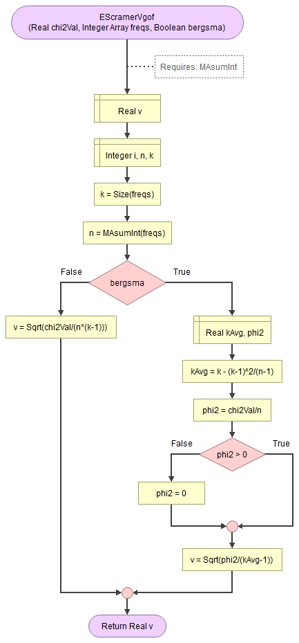
It takes as input the chi-square value, an array of integers with the observed frequencies, and a boolean to indicate to use the Bergsma correction.
It uses a small helper function to sum an array of integers.
Flowgorithm file: FL-EScramerVgof.fprg.
with Python
Jupyter Notebook from video: ES - Cramers V (GoF).ipynb.
Data file from video: GSS2012a.csv.
with R (Studio)
R script from video: ES - Cramers V (GoF).R.
Data file from video: Pearson Chi-square independence.csv.
with SPSS
Unfortunately SPSS does not have a method to determine Cramér's V directly from the GUI, however the calculation is not very difficult once you have the output from the previous part.
The video below shows how this could be done with a bit of help from Excel
Online calculator
Enter the requested information below:
Manually (formula and example)
Formula
The formula for Cramér's V is:
\(V=\sqrt\frac{\chi^{2}}{n\times df}\)
In the above formula \(\chi^2\) is the chi-square test value, \(n\) is the total sample size, and \(df\) is the degrees of freedom, determined by \(df=k-1\). \(k\) is the number of categories.
Example.
If we have a chi-square value of 1249.13, a total sample size of 1941, and had five categories, we can first determine the degrees of freedom (df):
\(df = k - 1 = 5 - 4 = 4\)
Then we can fill out all values in the formula for Cramér's V:
\(V=\sqrt\frac{\chi^{2}}{n\times df}=\sqrt\frac{1249.13}{1941\times4}=\sqrt\frac{1249.13}{7764}\approx\sqrt{0.1609}\approx0.4011\)
A correction can be applied using the procedure proposed by Bergsma (2013). This is actually for a Cramér’s V with a chi-square test of independence, but adapting it for a goodness-of-fit is possible.
Alternatives for Cramér's V as an effect size measure can also be Cohen's w, or Johnston-Berry-Mielke E.
One set of rule-of-thumb for Cramér's V with a goodness-of-fit test, is by converting it to Cohen's w and then use the rules of thumb from that. This will depend on the number of categories (k). In Table 1 the already converted rule of thumb.
| k | Negligible | Small | Medium | Large |
|---|---|---|---|---|
| 2 | 0 < 0.100 | 0.100 < 0.300 | 0.300 < 0.500 | ≥ 0.500 |
| 3 | 0 < 0.071 | 0.071 < 0.212 | 0.212 < 0.354 | ≥ 0.354 |
| 4 | 0 < 0.058 | 0.058 < 0.173 | 0.173 < 0.289 | ≥ 0.289 |
| 5 | 0 < 0.050 | 0.050 < 0.150 | 0.150 < 0.250 | ≥ 0.250 |
| k | 0.1 / SQRT(k-1) | 0.3 / SQRT(k-1) | 0.5 / SQRT(k-1) | |
| Note: Adapted from Statistical power analysis for the behavioral sciences (2nd ed., pp. 227) by J. Cohen, 1988, L. Erlbaum Associates. | ||||
In the example Cramér's V is 0.401 (see videos below on how to determine this), and we had 5 categories, which would indicate a large effect.
We could add this to our report:
A Pearson chi-square test of goodness-of-fit showed that the marital status was not equally distributed in the population, χ2(4, N = 1941) = 1249.13, p < .001, with a relatively strong (Cramér's V = .40) effect size according to conventions for Cramér's V (Cohen, 1988).
Step 5: Post-Hoc Analyses
The overall test can show if the proportions might be different for some categories in the population, but we often then would like to know, which categories are different. We can compare each possible pair of categories. In principle this makes it each time a binary variable, for which we can use a one-sample binomial test (or an alternative).
Because we are comparing multiple pairs, we run the risk of rejecting the assumption with a chance of 5% each time. This quickly adds up, and the chance of making the wrong decision at least once grows then rapidly. To counter this, we will need to adjust the pairwise test results a little. One common method is to use the Bonferroni procedure (Bonferroni, 1935). He simply suggested to divide the 5% by the number of tests that are being done, and use that then as the criteria.
Click here to see how to perform a pairwise binomial test
with Excel
Excel file from video: PH - Pairwise Binomial.xlsm.
with Python
Jupyter Notebook from video: PH - Pairwise Binomial.ipynb.
Data file from video: GSS2012a.csv.
with R (Studio)
R script from video: PH - Pairwise Binomial.R.
Data file from video: Pearson Chi-square independence.csv.
with SPSS
Data file used in video: GSS2012-Adjusted.sav.
Depending on the number of pairs tested and the results, summarizing the results can be easy or tricky. In the example all were significant, so we could add something like:
A post-hoc pairwise binomial test with Bonferroni correction of marital status showed that all proportions were significantly different from each other (p < .003).
In some situations, you might just want to show a table with all the results.
Step 6: Effect Size for Post-Hoc Analyses
Also for each of the pairwise comparisons, we need to report an appropriate effect size. Since the pairwise comparison was done using a one-sample binomial test, we can use the effect size, for that test: Cohen g.
Cohen g is simply the difference between the observed proportion, and 0.5. Cohen gave some rule of thumb to interpret this, shown in Table 2.
| |g| | Interpretation |
|---|---|
| 0.00 < 0.05 | Negligible |
| 0.05 < 0.15 | Small |
| 0.15 < 0.25 | Medium |
| 0.25 or more | Large |
| Note: Adapted from Statistical power analysis for the behavioral sciences (2nd ed., pp. 147-149) by J. Cohen, 1988, L. Erlbaum Associates. | |
Click here to see how to determine Cohen's g...
with Excel
Excel file from video: ES - Cohen g.xlsm.
with Flowgorithm
A basic implementation for Cohen g is shown in the flowchart in figure 1
Figure 2
Flowgorithm for Cohen g

It takes as input the frequency of one of the categories (k) and the sample size (n).
Flowgorithm file: ES - Cohen g.fprg.
with Python
Jupyter Notebook from video: ES - Cohen g.ipynb.
Datafile used in video: StudentStatistics.csv
with R (Studio)
R script from video: binary - effect sizes.R.
Datafile used in video: StudentStatistics.sav
with SPSS
Datafile used in video: StudentStatistics.sav
Online calculator
Enter the number of cases of the first category, then the total sample size:
Manually (using Formula)
Given a sample proportion (p) and the expected proportion in the population (π), the formula for Cohen's g will be:
\(g=p-\pi\)
The sample proportion in the example was 0.26 and the expected proportion was 0.50, in the example this therefor gives:
\(g=0.26-0.50=-0.24\)
Often the absolute value is used (the so-called nondirectional Cohen's g):
\(g=|0.26-0.50|=|-0.24|=0.24\)
The example will have the following results:
| Category 1 | Category 2 | n1 | n2 | total | proportion | Cohen g | size |
|---|---|---|---|---|---|---|---|
| married | widowed | 972 | 181 | 1153 | 0,843 | 0,3430 | large |
| married | divorced | 972 | 314 | 1286 | 0,7558 | 0,2558 | large |
| married | separated | 972 | 79 | 1051 | 0,9248 | 0,4248 | large |
| married | never married | 972 | 395 | 1367 | 0,711 | 0,2110 | medium |
| widowed | divorced | 181 | 314 | 495 | 0,3657 | 0,1343 | small |
| widowed | separated | 181 | 79 | 260 | 0,6962 | 0,1962 | medium |
| widowed | never married | 181 | 395 | 576 | 0,3142 | 0,1858 | medium |
| divorced | separated | 314 | 79 | 393 | 0,799 | 0,2990 | large |
| divorced | never married | 314 | 395 | 709 | 0,4429 | 0,05712 | small |
| separated | never married | 79 | 395 | 474 | 0,1667 | 0,3333 | large |
Summarizing this for the report can be tricky. We could do something as:
Married had a large difference with the other categories (g > 0.25), except for never married, which was medium (g = .21). The same goes for separated, which had a large difference with the other categories (g > 0.29), except for widowed, which was medium (g = 0.19). The differences between divorced with widowed and never married were each small (g < 0.14). Divorced vs. separated was another large difference (g = 0.40) and widowed was medium different from separated (g = 0.20).
It is still a lot of text, so if your research is focussed on a particular category, you might want to just describe that category, and refer to a table as Table 3 in an appendix.
Alternatives to Cohen g could be Cohen h' or the Alternative Ratio.
Step 7: Reporting
In each step, we already discussed how it could be reported. For the example used, the final report could have somthing like the following:
The media often reports that people are getting less often married these days. Figure 1 shows the results of the marital status in the survey.
Figure 1
Results of marital status
As can be seen Figure 1 almost 50% of the respondents is married and only a few were separated.
A Pearson chi-square test of goodness-of-fit showed that the marital status was not equally distributed in the population, χ2(4, N = 1941) = 1249.13, p < .001, with a relatively strong (Cramér's V = .40) effect size according to conventions for Cramér's V (Cohen, 1988).
A post-hoc pairwise binomial test with Bonferroni correction of marital status showed that all proportions were significantly different from each other (p < .003). Married had a large difference with the other categories (g > 0.25), except for never married, which was medium (g = .21). The same goes for separated, which had a large difference with the other categories (g > 0.29), except for widowed, which was medium (g = 0.19). The differences between divorced with widowed and never married were each small (g < 0.14). Divorced vs. separated was another large difference (g = 0.40) and widowed was medium different from separated (g = 0.20).
If you want to make things easy for yourself and are using Excel, Python or R, you can use my library/add-on to perform each step.
Using a stikpet Library/Add-On
Excel and the stikpetE add-on
Excel file from video: stikpetE - Single Nominal
Python and the stikpetP library
Notebook from video: stikpetP - Single Nominal.ipynb
R and the stikpetE library
Notebook from video: stikpetR - Single Nominal

Google adds