
Analyse a Single Scale Variable
The analysis of a single scale variable can be done with the steps shown below. Click on each step to reveal how this step can be done. As an example we are going to analyse the age variable of the results from a survey. Our guess is that the average age in the entire population is 49.
Step 1: Impression
The first step is to get a rough overview of the collected data. A frequency table is often then quite useful. However, with a scale variable this might become very long and therefor still not very clear. The 'trick' is to bin the scores (making the scores ordinal). To do this, we first need to decide on how many bins should be used.
Usually I try to aim myself to have between 4 and 10 bins, but there are various methods to decide on this.
Click here to see how you to determine the number of bins...
with R (Studio)
Notebook from video: IM - Binning (nr of bins) (R).ipynb
with stikpetR:
without stikpetR:
manually (formula's)
For the formula's below \(k\) is the number of bins, and \(n\) the sample size. The \(\left \lceil \dots \right \rceil\) is the ceiling function, which means to round up to the nearest integer
Square-Root Choice (Duda & Hart, 1973)
\( k = \left \lceil\sqrt{n}\right \rceil \)
Sturges (1926, p. 65)
\( k = \left\lceil\log_2\left(n\right)\right\rceil+1 \)
QuadRoot (anonymous as cited in Lohaka, 2007, p. 87)
\( k = 2.5\times\sqrt[4]{n} \)
Rice (Lane, n.d.)
\( k = \left\lceil 2\times\sqrt[3]{n} \right\rceil \)
Terrell and Scott (1985, p. 209)
\( k = \sqrt[3]{2\times n} \)
Exponential(Iman & Conover as cited in Lohaka, 2007, p. 87)
\( k = \left\lceil\log_2\left(n\right)\right\rceil \)
Velleman (Velleman, 1976 as cited in Lohaka 2007)
\( \begin{cases}2\times\sqrt{n} & \text{ if } n\leq 100 \\ 10\times\log_{10}\left(n\right) & \text{ if } n > 100\end{cases} \)
Doane(1976, p. 182)
\( k = 1 + \log_2\left(n\right) + \log_2\left(1+\frac{\left|g_1\right|}{\sigma_{g_1}}\right) \)
In the formula's \(g_1\) the 3rd moment skewness:
\( g_1 = \frac{\sum_{i=1}^n\left(x_i-\bar{x}\right)^3} {n\times\sigma^3} = \frac{1}{n}\times\sum_{i=1}^n\left(\frac{x_i-\bar{x}}{\sigma}\right)^3 \)
With \(\sigma = \sqrt{\frac{\sum_{i=1}^n\left(x_i-\bar{x}\right)^2}{n}}\)
The \(\sigma_{g_1}\) is defined using the formula:
\( \sigma_{g_1}=\sqrt{\frac{6\times\left(n-2\right)}{\left(n+1\right)\left(n+3\right)}} \)
Formula's that determine the width (h) for the bins
Using the width and the range, it can be used to determine the number of categories:
\( k = \frac{\text{max}\left(x\right)-\text{min}\left(x\right)}{h} \)
Scott (1979, p. 608)
\( h = \frac{3.49\times s}{\sqrt[3]{n}} \)
Where \(s\) is the sample standard deviation:
\(s = \sqrt{\frac{\sum_{i=1}^n\left(x_i-\bar{x}\right)^2}{n-1}}\)
Freedman-Diaconis (1981, p. 3)
\( h = 2\times\frac{\text{IQR}\left(x\right)}{\sqrt[3]{n}} \)
Where \( \text{IQR}\) the inter-quartile range.
A more complex technique is for example from Shimazaki and Shinomoto (2007). For this, we define a 'cost function' that needs to be minimized:
\( C_k = \frac{2\times\bar{f_k}-\sigma_{f_k}}{h^2} \)
With \(\bar{f_k}\) being the average of the frequencies when using \(k\) bins, and \(\sigma_{f_k}\) the population variance. In formula notation:
\(\bar{f_k}=\frac{\sum_{i=1}^k f_{i,k}}{k}\)
\(\sigma_{f_k}=\frac{\sum_{i=1}^k\left(f_{i,k}-\bar{f_k}\right)^2}{k}\)
Where \(f_{i,k}\) is the frequency of the i-th bin when using k bins.
Note that if the data are integers, it is recommended to use also bin widths that are integers.
Stone (1984, p. 3) is similar, but uses as a cost function:
\(C_k = \frac{1}{h}\times\left(\frac{2}{n-1}-\frac{n+1}{n-1}\times\sum_{i=1}^k\left(\frac{f_i}{n}\right)^2\right)\)
Knuth (2019, p. 8) suggest to use the k-value that maximizes:
\(P_k=n\times\ln\left(k\right) + \ln\Gamma\left(\frac{k}{2}\right) - k\times\ln\Gamma\left(\frac{1}{2}\right) - \ln\Gamma\left(n+\frac{k}{2}\right) + \sum_{i=1}^k\ln\Gamma\left(f_i+\frac{1}{2}\right)\)
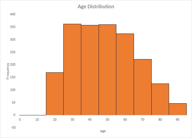
Once we have the bins, we can create a frequency table as shown in Table 1.
| Age | Frequency | Percent | Cumulative Percent |
|---|---|---|---|
| 15 < 25 | 170 | 9 | 9 |
| 25 < 35 | 363 | 18 | 27 |
| 35 < 45 | 358 | 18 | 45 |
| 45 < 55 | 360 | 18 | 64 |
| 55 < 65 | 324 | 16 | 80 |
| 65 < 75 | 222 | 11 | 91 |
| 75 < 85 | 125 | 6 | 98 |
| 85 < 95 | 47 | 2 | 100 |
| total | 1969 | 100 |
Click here to see how to create a frequency table with Excel, Python, R, or SPSS.
with Python
Jupyter Notebook of video is available here.
with stikpetP library
without stikpetP library
with R (Studio)
with stikpetP library
Jupyter Notebook of video is available here.
without stikpetR library
R script of video is available here.
Datafile used in video: GSS2012-Adjusted.sav
with SPSS
There are a three different ways to create a frequency table with SPSS.
An SPSS workbook with instructions of the first two can be found here.
using Frequencies
watch the video below, or download the pdf instructions (via bitly, opens in new window/tab).
Datafile used in video: Holiday Fair.sav
using Custom Tables
watch the video below, or download the pdf instructions for versions before 24, or version 24 (via bitly, opens in new window/tab)
Datafile used in video: Holiday Fair.sav
using descriptive shortcut
watch the video below, or download the pdf instructions (via bitly, opens in new window/tab).
Datafile used in video: StudentStatistics.sav
Note that because the bins are the same size, we do not need to determine so-called frequency densities.
From the table it appears the number of respondents drops gradually starting at 55 years, perhaps a visualisation makes this more clear.
Step 2: Visualisation
To visualise the results of a single scale variable we could create a histogram from the table made in step 1, as shown in Figure 1.
Figure 1.
Age distribution.
Click here to see how you to create a histogram
with Excel
Excel file from video: VI - Histogram (single) (E).xlsx
with equal bin widths (2016 or later)
with equal bin widths (before v. 2016)
with unequal bin widths
with SPSS
Four different methods to get a histogram with SPSS, using Chart-builder, Legacy Dialogs, Frequencies, or Explore. A video for each is below.
using Chart-builder
using Legacy Dialogs
using Frequencies
using Explore
When showing a chart it is good to also talk a little bit about it. For a scale variable you might want to describe the shape of the histogram. It of course always depends on your specific data, but inform your reader what you notice from the graph or what you want to show. In this example we get the same conclusion as we saw from the frequency table: it appears the number of respondents drops gradually starting at 55 years
An alternative could be a more technical visualisation known as a box-plot, or a stem-and-leaf plot.
Step 3: Statistical Measures
Our guess is that in the population the average age is 49 years. From the frequency table and histogram, this doesn't seem unreasonable, but we will need to test for this. Before we do this, it might actually be helpful to know what the average actually was in our sample.
The average (mean) alone is not very meaningful. If your head is in a burning oven and your feet are in a freezer, on average you are doing just fine. For this, measures of dispersion are also needed. The most commonly used measure of dispersion is probably the standard deviation.
In the example data, the sample mean was 48 years, and the standard deviation 17.69.
Click here to see how to determine the mean and standard deviation...
with Excel
Excel file from video: CEDI - Mean and Standard Deviation.xlsm.
with Flowgorithm
The Mean
A flowgorithm for the (arithmetic) mean in Figure 1.

It takes as input paramaters the scores.
It uses a function MAsumReal (sum of real values)
Flowgorithm file: FL-CEmean.fprg.
The Standard Deviation:
A flowgorithm for the sample standard deviation in Figure 1.

It takes as input paramaters the scores.
It uses the mean function (CEmean) and a function MAsumReal (sum of real values)
Flowgorithm file: FL-VAsd.fprg.
with Python
The Standard Deviation:
Jupyter Notebook from video: DI - Standard Deviation.ipynb.
with R
R script from video: CEDI - Mean and Standard Deviation.R.
with SPSS
There are a four different ways to determine the mean and standard deviation with SPSS.
using Frequencies
using Descriptives
using Explore
using a shortcut
Manually (Formulas)
The formula for the (arithmetic) mean is:
\(\bar{x} = \frac{\sum_{i=1}^n x_i}{n}\)
The formula for the (ubiased sample) standard deviation is:
\(s=\sqrt{\frac{\sum_{i=1}^n \left(x_i - \bar{x}\right)^2}{n-1}}\)
Where \(x_i\) is the i-th score, and \(n\) the sample size.
If your data is the entire population, the standard deviation is calculated by dividing by n instead of n - 1.
The standard deviation is roughly the average distance to the mean of all scores. Usually, lot of scores will be between mean and one standard deviation (about 68%). In the example this means a lot of scores will be between 48 - 17.69 and 48 + 17.69.
The expected age of 49 is not that far off from the sample mean.
Besides the arithmetic mean, there are quite a few different measures that could be used as a measure of center for a scale variable. For more information on these, see the Mean page. Similar as a measure of dispersion there are alternatives to the standard deviation. See the Quantitative Variation page for more information on these.
Step 4: Test
We got a decent impression of the sample data, but how about the population? That is where null-hypothesis significance testing comes in. One commonly used test for a single mean is the one-sample Student t-test.
Click here to see how you can perform this test
with Excel
Excel file from video: TS - Student t (one-sample) (E).xlsm
with stikpetE
without stikpetE
with Flowgorithm
A flowgorithm for the one-sample Student t-test in Figure 1.
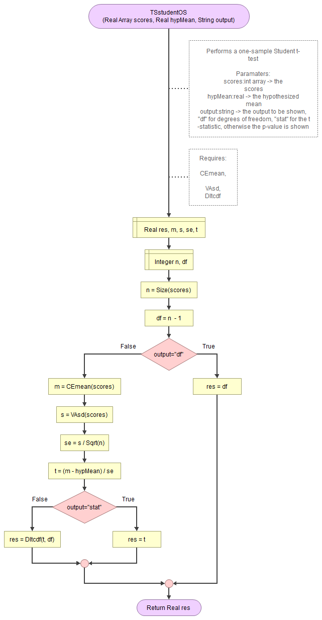
It takes as input the scores, the hypothesized mean, and a string for which output to show (df, statistic, or p-value).
It uses a function for the mean (CEmean), standard deviation (VAsd) and the t cumulative distribution (DItcdf). These in turn require the MAsumReal function (sums an array of real values) and the standard normal cumulative distribution (DIsncdf).
Flowgorithm file: FL-TSstudentOS.fprg.
with Python
Notebook from video: TS - Student t (one-sample) (P).ipynb
with stikpetP
without stikpetP
with SPSS
Formulas
Formula's
The t-value can be determined using:
\(t=\frac{\bar{x}-\mu_{H_{0}}}{SE}\)
In this formula \(\bar{x}\) is the sample mean, \(\mu_{H_0}\) the expected mean in the population (the mean according to the null hypothesis), and SE the standard error.
The standard error can be calculated using:
\(SE=\frac{s}{\sqrt{n}}\)
Where n is the sample size, and s the sample standard deviation.
The formula for the sample standard deviation is:
\(s=\sqrt{\frac{\sum_{i=1}^{n}\left(x_{i}-\bar{x}\right)^{2}}{n-1}}\)
In this formula xi is the i-th score, and n is the sample size.
The sample mean can be calculated using:
\(\bar{x}=\frac{\sum_{i=1}^{n}x_{i}}{n}\)
The degrees of freedom is determined by:
\(df=n-1\)
Where n is the sample size
Example (different example)
We are given the ages of five students, and have an hypothesized population mean of 24. The ages of the students are:
\(X=\left\{18,21,22,19,25\right\}\)
Since there are five students, we can also set n = 5, and the hypothesized population of 24 gives \(\mu_{H_{0}}=24\)
For the standard deviation, we first need to determine the sample mean:
\(\bar{x}=\frac{\sum_{i=1}^{n}x_{i}}{n}=\frac{\sum_{i=1}^{5}x_{i}}{5}=\frac{18+21+22+19+25}{5}\)
\(=\frac{105}{5}=21\)
Then we can determine the standard deviation:
\(s=\sqrt{\frac{\sum_{i=1}^{n}\left(x_{i}-\bar{x}\right)^{2}}{n-1}}=\sqrt{\frac{\sum_{i=1}^{5}\left(x_{i}-21\right)^{2}}{5-1}}=\sqrt{\frac{\sum_{i=1}^{5}\left(x_{i}-21\right)^{2}}{4}}\)
\(=\sqrt{\frac{\left(18-21\right)^{2}}{4}+\frac{\left(21-21\right)^{2}}{4}+\frac{\left(22-21\right)^{2}}{4}+\frac{\left(19-21\right)^{2}}{4}+\frac{\left(25-21\right)^{2}}{4}}\)
\(=\sqrt{\frac{\left(-3\right)^{2}}{4}+\frac{\left(0\right)^{2}}{4}+\frac{\left(1\right)^{2}}{4}+\frac{\left(-2\right)^{2}}{4}+\frac{\left(4\right)^{2}}{4}}\)
\(=\sqrt{\frac{9}{4}+\frac{0}{4}+\frac{1}{4}+\frac{4}{4}+\frac{16}{4}}=\sqrt{\frac{9+0+1+4+16}{4}}=\sqrt{\frac{30}{4}}\)
\(=\sqrt{\frac{15}{2}}=\frac{1}{2}\sqrt{15\times2}=\frac{1}{2}\sqrt{30}\approx2.74\)
The standard error then becomes:
\(SE=\frac{s}{\sqrt{n}}=\frac{\frac{1}{2}\sqrt{30}}{\sqrt{5}}=\frac{\frac{\sqrt{30}}{2}}{\sqrt{5}}=\frac{\sqrt{30}}{2\times\sqrt{5}}\)
\(=\frac{1}{2}\times\frac{\sqrt{30}}{\sqrt{5}}=\frac{1}{2}\times\sqrt\frac{30}{5}=\frac{1}{2}\sqrt{6}\approx1.22\)
The t-value:
\(t=\frac{\bar{x}-\mu_{H_{0}}}{SE}=\frac{21-24}{\frac{1}{2}\sqrt{6}}=\frac{-3}{\frac{\sqrt{6}}{2}}=\frac{-3\times2}{\sqrt{6}}=\frac{-6}{\sqrt{6}}\)
\(gif.latex?=\frac{-6}{\sqrt{6}}\times\frac{\sqrt{6}}{\sqrt{6}}=\frac{-6\times\sqrt{6}}{\sqrt{6}\times\sqrt{6}}=\frac{-6\times\sqrt{6}}{6}=-\sqrt{6}\approx-2.45\)
The degrees of freedom is relatively simple:
\(df=n-1=5-1=4\)
The two-sided significance is then usually found by using the t-value and the df, and consulting a t-distribution table, or using some software. If you really had to determine it manually, it would involve the formula for the t-distribution (the cumulative density function):
\(2\times\int_{x=|t|}^{\infty}\frac{\Gamma\left(\frac{df+1}{2}\right)}{\sqrt{df\times\pi}\times\Gamma\left(\frac{df}{2}\right)}\times\left(1+\frac{x^2}{df}\right)^{-\frac{df+1}{2}}\)
See the Student t-distribution section for more details.
The assumption about the population for this test, is that the mean in the population is a specified value, in our example 49 years. The most important result from the test is the p-value (significance). This is the probability of obtaining a result as in our sample, or even more extreme, if the assumption about the population would be correct. In the example this p-value is 0.043. This is below the usual threshold of 0.05. It is so unlikely to have a result as in our sample (or even more extreme) if the assumption about the population is true, that this assumption is most likely incorrect. The average age in the population is therefor most likely not 49 years old. We speak of a significant result if we have a p-value below the pre-set threshold (usually 0.05).
If the p-value would have been above the threshold, we do not claim the assumption to be true, we simply do not have enough evidence to reject it.
It might be a bit surprising, since our sample mean of 48 was not far off from the expected population mean of 49. The sample size though of 1969 is quite large, which can make small differences still become significant. Besides a significance test, we should therefor also determine an effect size measure.
The one-sample Student t-test is just one test that could be used, alternatives are a one-sample z-test, or a one-sample trimmed mean test.
Step 5: Effect Size
The last step before we write up all results, is to add an effect size measure. Hedges g is one possible effect size measure to use with a one-sample t-test.
Click here to see how to obtain Hedges g for a one-sample test.
with Flowgorithm
A flowgorithm for Hedges g (one-sample) in Figure 1.

It takes as input paramaters the scores, the hypothesized mean, and which approximation to use (if any).
It uses a function for Cohen's d (EScohenDos), the gamma function (MAgamma), and the e power function (MAexp). Cohen's d function requires in turn the mean (CEmean) and standard deviation (VAsd) functions, which make use of the MAsumReal (sum of real values) function. The gamma function needs the factorial function (MAfact)
Flowgorithm file: FL-EShedgesGos.fprg.
with Python
Jupyter Notebook used in video: ES - Hedges g (one-sample) (P).ipynb.
without stikpetP library
with R (Studio)
Jupyter Notebook used in video: ES - Hedges g (one-sample) (R).ipynb.
video to be uploaded
with SPSS
This has become available in SPSS 27. There is no option in earlier versions of SPSS to determine Hedges g, but it can easily be calculated using the 'Compute variable' option as shown in the video.
SPSS 27 or later
Datafile used in video: GSS2012-Adjusted.sav
SPSS 26 or earlier
Datafile used in video: GSS2012-Adjusted.sav
manually (Formula)
The exact formula for Hedges g is (Hedges, 1981, p. 111):
\(g = d\times\frac{\Gamma\left(m\right)}{\Gamma\left(m-0.5\right)\times\sqrt{m}}\)
With \(d\) as Cohen's d, and \(m = \frac{df}{2}\), where \(df=n-1\)
The \(\Gamma\) indicates the gamma function, defined as:
\(\Gamma\left(a=\frac{x}{2}\right)=\begin{cases} \left(a - 1\right)! & \text{ if } x \text{ is even}\\ \frac{\left(2\times a\right)!}{4^a\times a!}\times\sqrt{\pi} & \text{ if } x \text{ is odd}\end{cases}\)
Because the gamma function is computational heavy there are a few different approximations.
Hedges himself proposed (Hedges, 1981, p. 114):
\(g^* \approx d\times\left(1 - \frac{3}{4\times df-1}\right)\)
Durlak (2009, p. 927) shows another factor to adjust Cohens d with:
\(g^* = d\times\frac{n-3}{n-2.25}\times\sqrt{\frac{n-2}{n}}\)
Xue (2020, p. 3) gave an improved approximation using:
\(g^* = d\times\sqrt[12]{1-\frac{9}{df}+\frac{69}{2\times df^2}-\frac{72}{df^3}+\frac{687}{8\times df^4}-\frac{441}{8\times df^5}+\frac{247}{16\times df^6}}\)
Note 1. You might come across the following approximation: (Hedges & Olkin, 1985, p. 81)
\(g^* = d\times\left(1-\frac{3}{4\times n - 9}\right)\)
This is an alternative but equal method, but for the paired version. In the paired version we set df = n - 2, and if we substitute this in the Hedges version it gives the same result. The denominator of the fraction will then be:
\(4\times df - 1 = 4 \times\left(n-2\right) - 1 = 4\times n-4\times2 - 1 = 4\times n - 8 - 1 = 4\times n - 9\)
Note 2. Often for the exact formula 'm' is used for the degrees of freedom, and the formula will look like:
\(g = d\times\frac{\Gamma\left(\frac{m}{2}\right)}{\Gamma\left(\frac{m-1}{2}\right)\times\sqrt{\frac{m}{2}}}\)
Note 3: Alternatively the natural logarithm gamma can be used by using:
\(j = \ln\Gamma\left(m\right) - 0.5\times\ln\left(m\right) - \ln\Gamma\left(m-0.5\right)\)
and then calculate:
\(g = d\times e^{j}\)
In the formula for \(j\) we still use \(m = \frac{df}{2}\).
Hedges g can range from negative infinity to positive infinity. A zero would indicate no difference at all between the two means, the higher the value the larger the effect. In the example, Hedges g is 0.1021.
Various authors have proposed rules-of-thumb for the classification of Cohen d, and since Hedges g is a correction for Cohen d, we could use the same classifications. A few are listed in table 2.
| |d| | Brydges (2019, p. 5) | Cohen (1988, p. 40) | Sawilowsky (2009, p. 599) | Rosenthal (1996, p. 45) | Lovakov and Agadullina (2021, p. 501) |
|---|---|---|---|---|---|
| 0.00 < 0.10 | negligible | negligible | negligible | negligible | negligible |
| 0.10 < 0.15 | very small | ||||
| 0.15 < 0.20 | small | small | |||
| 0.20 < 0.35 | small | small | small | ||
| 0.35 < 0.40 | medium | ||||
| 0.40 < 0.50 | medium | ||||
| 0.50 < 0.65 | medium | medium | medium | ||
| 0.65 < 0.75 | large | ||||
| 0.75 < 0.80 | large | ||||
| 0.80 < 1.20 | large | large | large | ||
| 1.20 < 1.30 | very large | ||||
| 1.30 < 2.00 | very large | ||||
| 2.00 or more | huge |
Note that these are just some rule-of-thumb and can differ depending on the field of the research.
The Hedges g of 0.1021 in the example would therefor be classified as negligible. So even though the population age is significantly different from 49, it isn't much different.
Hedges g is a correction for Cohen's d', but Cohen's d' itself could of course also be used.
Step 6: Reporting
The last step is of course to report all our findings. Here is how I would do this.
I like to start with a visualisation, but use an IST model for this: Introduce - Show - Tell. First a small introduction, then show the visualisation and then talk about it. Do not use 'see figure below', but simply refer to the figure number.
The visualisation is about the sample, so next is the inference: the result of the test. The basic format is the letter of the distribution the test uses (in this case a t-distribution), then between parenthesis the degrees of freedom (in this case the sample size minus 1), equals the test statistic (in this case the t-value), and then the p-value in three decimals. If the p-value is below .001 you can simply use < .001. For commonly tests you do not need to give the reference of the original author of the test.
Last is probably most important, to write a conclusion in terms also non-statisticians can understand.
In the example, this would look something as below:
In our previous report management noted that the average age of our customers is 49 years old, but no data was shown. A survey was held at our local shop among the customers asking them about their age. The survey results are shown in figure 1.
Figure 1.
Age distribution.
As can be seen from the histogram, there seems to be a decline in number of customers after 55 years old. The average aga in the sample was 48 years with a standard deviation of 17.69.
A one-sample Student t-test showed that the mean age of customers was significantly different from 49 at a .05 significance level, t(1968) = -2.02, p = .043. However the effect size was negligible, Hedges g = 0.1021.
Although the mean age will most likely not be 49 years old, it will not be far off.
If you want to make things easy for yourself and are using Excel, Python or R, you can use my library/add-on to perform each step.
Using a stikpet Library/Add-On
Excel and the stikpetE add-on
Excel file from video: stikpetE - Single Scale.xlsm
Python and the stikpetP library
Notebook from video: stikpetP - Single Scale.ipynb
R and the stikpetE library
Notebook from video: stikpetR - Single Scale.ipynb
Google adds