
One-Sample Wilcoxon Signed Rank Test
Introduction
The Wilcoxon Signed Rank (WSR) test (Wilcoxon, 1945) is often used to test a hypothesized median. There is also a sign-test that can test for a specified median. The WSR does not require the data to come from a normal distribution, but does need the data to come from a symmetrical distribution (Li & Johnson, 2014). The one-sample sign test doesn't have this condition, but is less powerful.
We could use it for example if people gave their opinion on something on a scale of fully disagree to fully agree, to test if in the population the median is signficantly different from the neutral score.
The test ranks the scores and compares the sum of the ranks of those scores that are above the hypothesized median, with those that are below. The name of this test is then the creator Wilcoxon, Signed because it looks at the sign of score minus hypothesized median, and Rank because it looks at the rank of the scores.
There also quite a few different variations on the test itself. See the Variations section for these. An independent samples version is also possible, but then named the Wilcoxon Rank Sum test, which is then the same as a Mann-Whitney U test. With paired data the Wilcoxon Signed Rank test can also be used.
Performing the Test
with Excel
Excel file from video: TS - Wilcoxon (One-Sample) (E).xlsm.
with stikpetE
without stikpetE
with Flowgorithm
exact test
WARNING: This very quickly becomes too large in computation that Flowgorithm can handle.
A flowgorithm for the exact one-sample Wilcoxon signed rank test is shown in Figure 1.
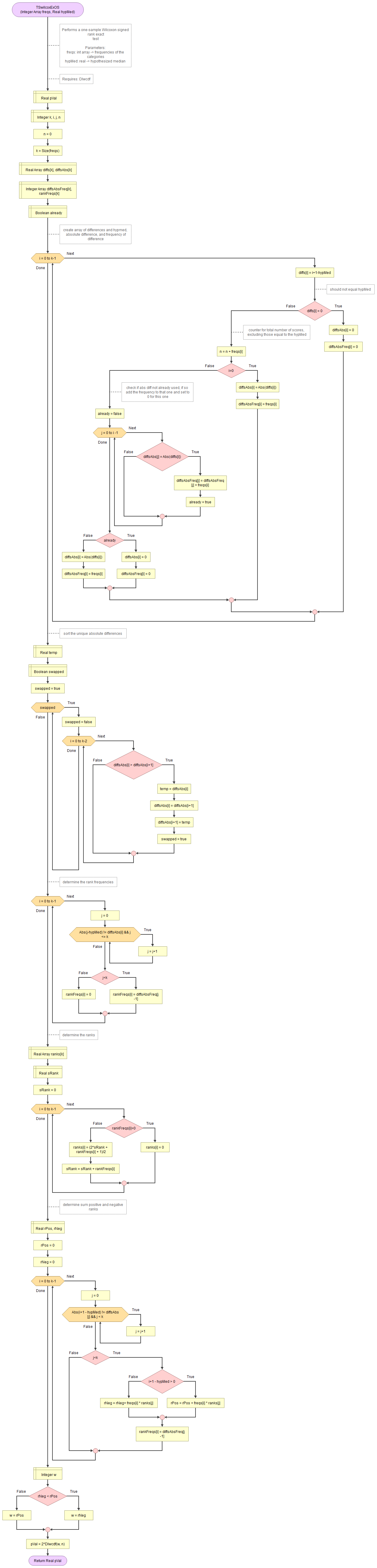
It takes as input an array of integers with the observed frequencies and the hypothesized median.
It uses the function for Wilcoxon distribution which in turn uses the permutation distribution and the binomial coefficient.
Flowgorithm file: FL-TSwilcoxOSexact.fprg.
normal approximation
A flowgorithm for the one-sample Wilcoxon signed rank test using the normal approximation is shown in Figure 2.
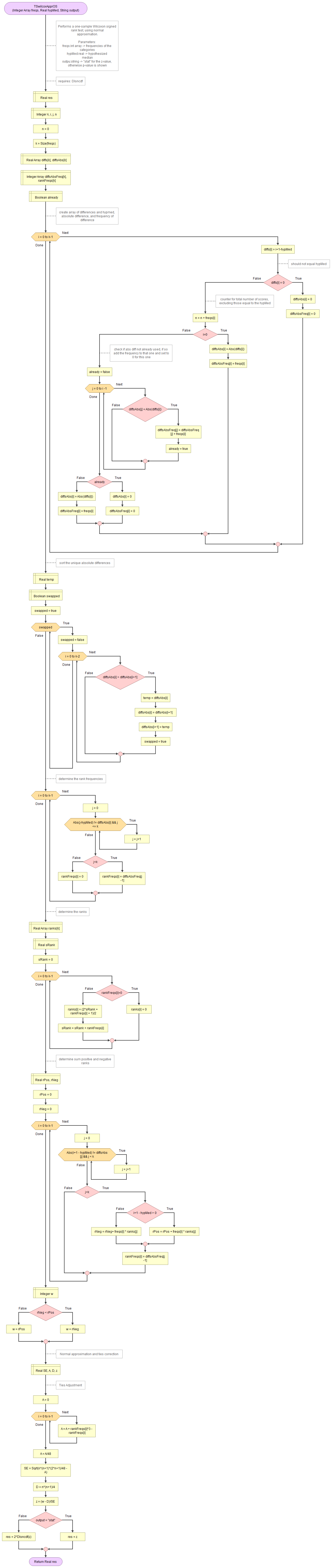
It takes as input an array of integers with the observed frequencies, the hypothesized median, and a string to indicate if you want to see the z-value or the p-value.
It uses the function for standard normal cumulative distribution.
Flowgorithm file: FL-TSwilcoxOSappr.fprg.
with Python
Jupyter Notebook from videos: TS - Wilcoxon (One-Sample) (P).ipynb.
with stikpetP
without stikpetP
with R
Jupyter Notebook from videos: TS - Wilcoxon (One-Sample) (R).ipynb.
with stikpetR
without stikpetR
Formulas
The unadjusted test statistic is given by:
\(T=\sum_{i=1}^{n_{r}^{+}}r_{i}^{+}\)
With:
- \(r=\text{rank}(|d|)\)
- \(d_{i}=y_{i}-\theta\)
Symbols used:
- \(n_{r}^{+}\) is the number of ranks with a positive deviation from the hypothesized median
- \(r_{i}^{+}\) the i-th rank of the ranks with a positive deviation from the hypothesized median
- \(\theta\) is the median tested (the hypothesized median).
- \(y_i\) is the i-th score of the variable after removing scores that were equal to \(\theta\)
If there are no ties, an exact method can be used, using the Wilcoxon Signed Rank Distribution.
Approximations
If the sample size is large enough, we can use a normal approximation. What is large enough varies quite per author. A few examples: n > 8 (slideplayer, 2015), n > 15 (SigMaxl, n.d.), n > 20 (Wikipedia, n.d.), n > 25 (Harris & Hardin, 2013), n > 30 (Winthrop, n.d.).
The z-statistic is given by:
\(Z = \frac{T - \mu_T}{\sigma_T}\)
or with a ties correction:
\(Z_{adj} = \frac{T - \mu_T}{\sigma_T^*}\)
With:
- \(\mu_T = \frac{n_r\times\left(n_r + 1\right)}{4}\)
- \(\sigma_T^2 = \frac{n_r\times\left(n_r + 1\right)\times\left(2\times n_r + 1\right)}{24}\)
- \(\sigma_T^{*2} = \sigma_T^2 - A\)
- \(A = \frac{\sum_{i=1}^k \left(t_i^3 - t_i\right)}{48}\)
Additional symbols used:
- \(n_{r}\) is the number of ranks used
- \(k\) the number of unique ranks
- \(t_i\) the frequency of the i-th unique rank
A Yates continuity correction can simply be applied:
In case of no ties:
\(Z = \frac{\left|T - \mu_T\right| - 0.5}{\sigma_T}\)
In case of ties:
\(Z_{adj} = \frac{\left|T - \mu_T\right| - 0.5}{\sigma_T^*}\)
An alternative approximation using the Student t distribution is given by Iman (1974, p. 799). The formula is:
\(t = \frac{T - \mu_T}{\sqrt{\frac{\sigma_T^2\times n_r - \left(T - \mu_T\right)^2}{n_r - 1}}}\)
or with the ties correction:
\(t = \frac{T - \mu_T}{\sqrt{\frac{\sigma_T^{*2}\times n_r - \left(T - \mu_T\right)^2}{n_r - 1}}}\)
The two versions for with a continuity correction are:
No ties correction, but continuity:
\(t = \frac{\left|T - \mu_T\right| - 0.5}{\sqrt{\frac{\sigma_T^2\times n_r - \left(\left|T - \mu_T\right| - 0.5\right)^2}{n_r - 1}}}\)
Both corrections:
\(t = \frac{\left|T - \mu_T\right| - 0.5}{\sqrt{\frac{\sigma_T^{*2}\times n_r - \left(\left|T - \mu_T\right| - 0.5\right)^2}{n_r - 1}}}\)
Iman (1974, p. 803) also provides a combination of the t-approximation and the regular z-approximation. The equation is given by:
\(Z_{I} = \frac{Z}{2}\times\left(1 + \sqrt{\frac{n_r - 1}{n_r - Z^2}}\right)\)
The \(Z\) is any of the previous methods.
Ties with mu
The default removes first any scores that are equal to the hypothesized median. There are two alternative methods for this. Both re-define \(d_i\) to:
\(d_i = x_i - \theta\)
Where \(x_i\) is simply the i-th score.
For the z-split method we only need to re-define:
\(T = \frac{\sum_{i=1}^{n_{d_0}}r_{i,0}}{2} + \sum_{i=1}^{n_{r}^{+}}r_{i}^{+}\)
Where \(n_{d_0}\) is the number of scores that equal the hypothesized median, and \(r_{i,0}\) is the rank of the i-th score that equals the hypothesized median.
In essence we added half the sum of the ranks that were equal to the hypothesized median.
For the z-split method all other calculations than go the same.
For the Pratt (1959) method we also re-define:
\(\mu_T = \frac{n_r\times\left(n_r + 1\right) - n_{d_0}\times\left(n_{d_0} + 1\right)}{4}\)
\(\sigma_T^2 = \frac{n_r\times\left(n_r + 1\right)\times\left(2\times n_r + 1\right) - n_{d_0}\times\left(n_{d_0} + 1\right)\times\left(2\times n_{d_0} + 1\right)}{24}\)
For the Pratt method, the ties correction still excludes the ties for the scores that equal the hypothesized median, but for the z-split method it will include them.
For both methods now \(n_r=n\), where n is the number of scores.
The Pratt (1959)a method and z-split method were found in Python’s documentation for scipy’s Wilcoxon function (scipy, n.d.). They also refer to Cureton (1967) for the Pratt method.
Interpreting the Result
The assumption about the population for this test (the null hypothesis) is that the median is a specific value.
The test provides a p-value, which is the probability of a test statistic as from the sample, or even more extreme, if the assumption about the population would be true. If this p-value (significance) is below a pre-defined threshold (the significance level \(\alpha\) ), the assumption about the population is rejected. We then speak of a (statistically) significant result. The threshold is usually set at 0.05. Anything below is then considered low.
If the assumption is rejected, we conclude that the median in the population will be different than the one used in the test.
Note that if we do not reject the assumption, it does not mean we accept it, we simply state that there is insufficient evidence to reject it.
Writing the results
Writing up the results of the test will depend on the method used. If an normal approximation is used (APA, 2019 p. 182):
z = <z-value>, p = <p-value>
If a Student t approximation is used (APA, 2019 p. 182):
t(<degrees of freedom>) = <t-value>, p = <p-value>
With an exact test, unfortunately APA doesn't mention an example for something using a Wilcoxon Distribution, but staying in line with the other distributions:
T(<sample size>) = <T-value>, p = <p-value>
So for example if a normal distribution was used:
A one-sample Wilcoxon Signed Rank test, with normal approximation, ties-correction and Pratt method for dealing with ties, indicated that the median was significantly different from the neutral option, z = 3.10, p < .001.
The p-value is shown with three decimal places, and no 0 before the decimal sign. If the p-value is below .0005, it can be reported as p < .001.
APA (2019, p. 88) states to also report an effect size measure.
Variations
There quite a few different variations possible on the test itself.
- Distribution to use
The exact test uses the Wilcoxon distribution, but this can be approximated using the normal distribution or t-distribution. - Ties with other scores
If the data contains scores that are equal to each other (tied) a ties correction should be used.
- Ties with hypothesized median
The original version simply started with removing all scores equal to the hypothesized median, but alternative methods also exist for this the z-split and Pratt method.
Google adds