
Analyse a Single Ordinal Variable
The analysis of a single ordinal variable can be done with the steps shown below. Click on each step to reveal how this step can be done.
Step 1: Impression
To begin with analysing a single ordinal variable, a good starting point can be to generate a frequency table, such as the one shown in Table 1.
| Frequency | Percent | Valid Percent | Cumulative Percent | ||
|---|---|---|---|---|---|
| Valid | very scientific | 100 |
5.1 |
10.5 |
10.5 |
| pretty scientific | 199 |
10.1 |
20.9 |
31.3 |
|
| not too scientific | 348 |
17.6 |
36.5 |
67.8 |
|
| not scientific at all | 307 |
15.6 |
32.2 |
100 |
|
| Subtotal | 954 |
48.3 |
100.0 |
||
| Missing | No answer | 1020 |
51.7 |
||
| Subtotal | 1020 |
51.7 |
|||
| Total | 1974 |
100.0 |
Click here to see how to create a frequency table with Excel, Python, R (Studio), or SPSS.
with Excel
File used in video: IM - Frequency Table (Ordinal).xlsm
with Python
File used in video: IM - Frequency Table.ipynb
Data file used in video and notebook GSS2012a.csv.
with SPSS
There are a three different ways to create a frequency table with SPSS.using Frequencies
watch the video below, or download the pdf instructions (via bitly, opens in new window/tab).
Datafile used in video: Holiday Fair.sav
using Custom Tables
watch the video below, or download the pdf instructions for versions before 24, or version 24 (via bitly, opens in new window/tab)
Datafile used in video: Holiday Fair.sav
using descriptive shortcut
watch the video below, or download the pdf instructions (via bitly, opens in new window/tab).
Datafile used in video: StudentStatistics.sav
See the explanation of frequency table for details on how to read this kind of table.
In the example we can see from the cumulative percent of only 31.3 that about 31% of the respondents think accounting is scientific. The table itself might not end up in the report, but gives a quick impression for yourself. Most would probably prefer a visualisation though.
Step 2: Visualisation
To take advantage of having an order with an ordinal variable, a stacked (a.k.a. compound) bar chart could be a useful visualisation. An example is shown in figure 1.
Figure 1.
Example of a compound bar-chart of a single ordinal variable

Click here to see how to create a stacked bar-chart
with Excel
Excel file from video: VI - Bar Chart (Stacked - Single).xlsm.
with Python
Jupyter Notebook used in video: VI - Bar Chart - Stacked Single Variable.ipynb.
Data file used in video and notebook GSS2012a.csv.
with R
R script used in video: VI - Bar Chart (Single Stack).R.
Data file used in video and notebook GSS2012a.csv.
with SPSS
Datafile used in video: GSS2012-Adjusted.sav
In the report I recommend using a ‘Introduce – Show – Tell’ approach. Introduce the figure, then show the figure, then talk about what you notice. From figure 1 we can see the same result as we already saw with the frequency table, but of course now visually. The respondents don't seem to find accounting very scientific. Is the result however significant? This will be the next step.
An alternative for a stacked bar-chart can be a dual-axis bar-chart, or in case there were many options to choose from in the ordinal variable a box-plot.
Step 3: Testing
With a single ordinal variable, we can test if in the population the score in the middle (median) will be a specific value. The value to be tested is often chosen to be the middle option of the possible values (the 'neutral' option). A one-sample Wilcoxon signed rank test can do this for us.
The null hypothesis (assumption about the population) is that the middle score in the population is X. In the example we can set X to between 'pretty scientific' and 'not too scientific', these were each coded as 2 and 3 resp. so we can use as our assumption: the middle score in the population is 2.5.
Click here to see how you can perform a one-sample Wilcoxon signed rank test.
with Excel
Excel file from video: TS - One-Sample Wilcoxon.xlsm.
with Flowgorithm
exact test
WARNING: This very quickly becomes too large in computation that Flowgorithm can handle.
A flowgorithm for the exact one-sample Wilcoxon signed rank test is shown in Figure 1.
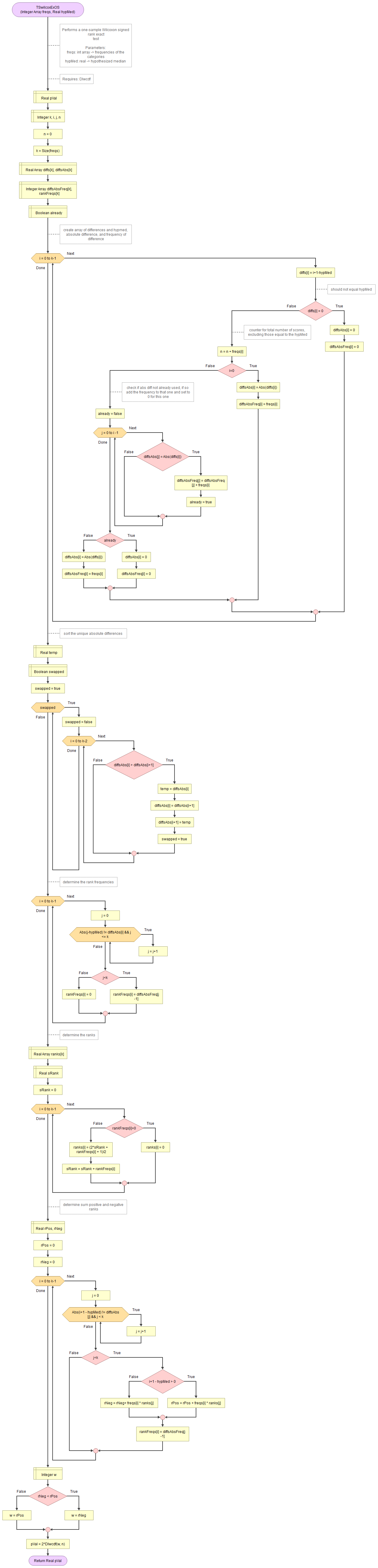
It takes as input an array of integers with the observed frequencies and the hypothesized median.
It uses the function for Wilcoxon distribution which in turn uses the permutation distribution and the binomial coefficient.
Flowgorithm file: FL-TSwilcoxOSexact.fprg.
normal approximation
A flowgorithm for the one-sample Wilcoxon signed rank test using the normal approximation is shown in Figure 2.
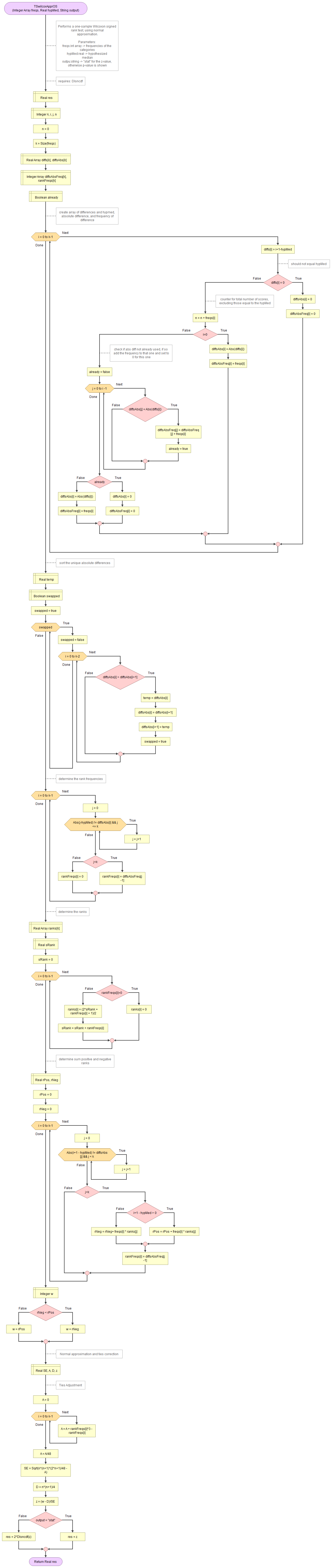
It takes as input an array of integers with the observed frequencies, the hypothesized median, and a string to indicate if you want to see the z-value or the p-value.
It uses the function for standard normal cumulative distribution.
Flowgorithm file: FL-TSwilcoxOSappr.fprg.
with Python
Jupyter Notebook used in video: TS - Wilcoxon One-Sample.ipynb.
Data file used in video and notebook GSS2012a.csv.
with R (Studio)
click on the thumbnail below to see where to find the values used in the report.
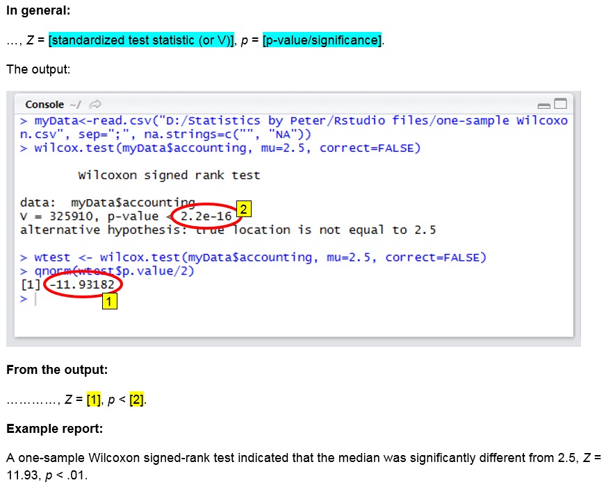
R script used in video: TS - One-Sample Wilcoxon.R.
Data file used in video and notebook GSS2012a.csv.
with SPSS
watch the video below, or download the pdf instructions (via bitly, opens in new window/tab).
click on the thumbnail below to see where to find the values used in the report.
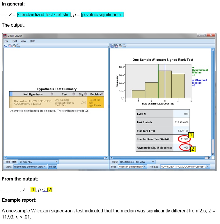
Datafile used in video: GSS2012-Adjusted.sav
Manually (formulas and example)
Formulas
The unadjusted test statistic is given by:
\( W=\sum_{i=1}^{n_{r}^{+}}r_{i}^{+} \)
In this formula \( n_{r}^{+}\) is the number of ranks with a positive deviation from the hypothesized median, and \(r_{i}^{+}\) the i-th rank of of the ranks with a positive deviation from the hypothesized median.
The ranks are based on the absolute deviation of each score with the hypothesized median, removing scores that are equal to the hypothesized median. In formula notation we could determine the sequence of ranks as:
\(r=\textup{rank}(|d|)\)
Where d is the sequence of:
\(d_{i}=y_{i}-\theta\)
Where θ is the hypothesized median, and and y the sequence of original scores, but with the scores removed that equal θ
To adjust for ties we need a few more things.
The variance is given by:
\( s^{2}=\frac{n_{r}\times\left(n_{r}+1\right)\times\left(2\times n_{r}+1\right)}{24} \)
Where nr is the number of ranks.
The adjustment is given by:
\(A=\frac{\sum_{i=1}^{n_f}\left(t_i^3-t_i\right)}{48}\)
In this formula ti is the number of ties for each unique ranks i, and nf the number of unique ranks.
The adjusted variance then becomes:
\(s_*^2=s^2-A\)
The adjusted standard error:
\(SE_*=\sqrt{s_*^2}\)
Another small adjustment is needed:
\(D=\frac{n_r\times\left(n_r+1\right)}{4}\)
Finally the adjusted W statistics is then:
\(W_*=\frac{W-D}{SE_*}\)
Example
We are given six scores from an ordinal scale and like to test if the median is significantly different from 3. The six scores are:
\(x=\left(4,4,5,1,5,3 \right)\)
The hypothesized median was given to be 3, so:
\(\theta=3\)
First we now remove any score from x that is equal to the hypothesized median, which in the example is only the last score. So we set:
\(y=\left(4,4,5,1,5\right)\)
Then we determine the difference with the hypothesized median:
\(d=\left(4-3,4-3,5-3,1-3,5-3\right)=\left(1,1,2,-2,2\right)\)
To determine the ranks, we need tha absolute values of these:
\(|d|=\left(|1|,|1|,|2|,|-2|,|2|\right)=\left(1,1,2,2,2\right)\)
Then we rank these absolute differences. The lowest score is a 1, but this occurs twice. So they take up rank 1 and 2, or on average rank 1.5. Then we have a score of 2, but this occurs three times. So they take ranks 3, 4 and 5, or on average rank 4. It is these average ranks that we need:
\(r=\left(1.5,1.5,4,4,4\right)\)
To determine the unadjusted W we sum up the ranks, but only for those that had a positive deviation (from d). The fourth entry in d is negative (-2), so we do not add the rank of 4 from that score. We therefor get:
\(W=1.5+1.5+4+4=11\)
We have five ranks so nr = 5, so we can also determine the variance:
\(s^2=\frac{n_{r}\times\left(n_{r}+1\right)\times\left(2\times n_{r}+1\right)}{24} =\frac{5\times\left(5+1\right)\times\left(2\times 5+1\right)}{24}\)
\(=\frac{5\times6\times\left(10+1\right)}{24}=\frac{5\times6\times11}{24}=\frac{330}{24}=\frac{55}{4}=13.75\)
We have a rank of 1.5 that occurs twice, and a rank of 4 that occurs three times. Therefore:
\(A=\frac{\sum_{i=1}^{n_f}\left(t_i^3-t_i\right)}{48}=\frac{\left(2^3-2\right)+\left(3^3-3\right)}{48} =\frac{\left(8-2\right)+\left(27-3\right)}{48} =\frac{6+24}{48}\)
\(=\frac{30}{48}=\frac{5}{8}=0.625\)
The adjusted variance then becomes:
\(s_*^2=s^2-A=\frac{55}{4}-\frac{5}{8}=\frac{55\times2}{4\times2}-\frac{5}{8}\)
\(=\frac{110}{8}-\frac{5}{8}=\frac{110-5}{8}=\frac{105}{8}=13.125\)
The adjusted standard error:
\(SE_*=\sqrt{s_*^2}=\sqrt\frac{105}{8}=\frac{1}{8}\sqrt{105\times8}=\frac{1}{8}\sqrt{840}\)
\(=\frac{1}{8}\sqrt{4\times210}=\frac{1}{8}\times\sqrt{4}\times\sqrt{210}=\frac{1}{8}\times2\times\sqrt{210}=\frac{1\times2}{8}\times\sqrt{210}\)
\(=\frac{2}{8}\times\sqrt{210}=\frac{1}{4}\sqrt{210}\approx3.623\)
The other small adjustment:
\(D=\frac{n_r\times\left(n_r+1\right)}{4}=\frac{5\times\left(5+1\right)}{4}=\frac{5\times6}{4}=\frac{30}{4}=\frac{15}{2}=7.5\)
The adjusted W statistic becomes:
\(W_*=\frac{W-D}{SE_*}=\frac{11-\frac{15}{2}}{\frac{1}{4}\sqrt{210}} =\frac{\frac{22}{2}-\frac{15}{2}}{\frac{\sqrt{210}}{4}} =\frac{\frac{22-15}{2}}{\frac{\sqrt{210}}{4}} =\frac{\frac{7}{2}}{\frac{\sqrt{210}}{4}}\)
\(=\frac{7\times4}{\sqrt{210}\times2} =\frac{7\times2}{\sqrt{210}} =\frac{14}{\sqrt{210}} =\frac{14}{\sqrt{210}}\times\frac{\sqrt{210}}{\sqrt{210}}\)
\(=\frac{14\times\sqrt{210}}{\sqrt{210}\times\sqrt{210}} =\frac{14\times\sqrt{210}}{210} =\frac{14\times\sqrt{210}}{14\times15} =\frac{\sqrt{210}}{15}\approx0.966\)
To determine the two-tailed significance either the exact Wilcoxon distribution is used, or if there is sufficient data the standard normal distribution is used.
In the results you will find a p-value (significance). This is the chance of obtaining a result as in the sample, or more extreme, if the assumption about the population is true. If this is a small chance (usually below .05) we would reject the assumption, otherwise we state we do not have enough evidence to reject it.
In the example, the p-value is .000, indicating that it is very very small. It is then below .05, so we reject the assumption. The assumption was that in the population the middle score will be at neutral, since we reject this we can assume it isn't. This indicates it must be in the population above or below the neutral. From the visualisation we can tell it will be below. So we can conclude that people tend to find accounting not so scientific.
Usually the Wilcoxon test is done with a standard normal distribution approximation, which means that for reporting the results we can use the following template:
z = <std. test statistic>, p = <p-value(sig.)>.
This is then preceded by the test and interpertation. In the example this could look like:
A one-sample Wilcoxon signed-rank test indicated that the median was significantly different from 2.5, Z = 11.93, p < .001.
An alternative for the one-sample Wilcoxon signed rank test can be a one-sample sign test, or a one-sample trinomial test.
The test only informs us if the results can be translated to the population, but not how strong/big the deviation is from the assumption. For this we need an effect size measure...
Step 4: Effect Size
One possible effect size measures that could be suitable for the one-sample Wilcoxon test, is dividing the z-value by the square root of the sample size (Fritz et al., 2012, p. 12; Mangiafico, 2016; Simone, 2017; Tomczak, M., & Tomczak, E., 2014, p. 23; ). I'll refer to this as the Rosenthal Correlation Coefficient (Rosenthal, 1991, p. 19).
Click here to see how you can obtain the Rosenthal Coefficient...
with Excel
Excel file: ES - Rosenthal Correlation.xlsm
with Flowgorithm
A flowgorithm for the Rosenthal Correlation in Figure 1.

It takes as input the z-value and an array of integers with the observed frequencies.
It uses the function a small helper function to determine the sum of an array.
Flowgorithm file: FL-ESrosenthal.fprg.
with Python
Jupyter Notebook: ES - Rosenthal Correlation.ipynb
with R (studio)
video to be uploaded
R script: ES - Rosenthal Correlation (one-sample).R
Data file: GSS2012a.csv.
with SPSS
Data file: GSS2012-Adjusted.sav
with an online calculator
Enter the standardized test statistic, and the sample size:
manually (Formula and Example)
Formula
The formula to determine the Rosenthal Correlation Coefficient is:
\(r_{Rosenthal}=\frac{Z}{\sqrt{n}}\)
In this formula Z is the Z-statistic, which in the case of a Wilcoxon one-sample test is the adjusted W statistic, and n the sample size.
Example
Note this is a different example than used in this section.
We are given six scores from an ordinal scale and like to test if the median is significantly different from 3. The six scores are:
\(x=\left(4,4,5,1,5,3 \right )\)
In the previous section we already calculated the adjusted W statistic, so we can set:
\(Z=W_*=\frac{\sqrt{210}}{15}\approx0.966\)
Since there are six scores we also know:
\(n=6\)
Filling out the formula for the Rosenthal Correlation, we then get:
\(r_{Rosenthal}=\frac{Z}{\sqrt{n}}=\frac{\frac{\sqrt{210}}{15}}{\sqrt{6}}=\frac{\sqrt{210}}{15\times\sqrt{6}}=\frac{1}{15}\times\frac{\sqrt{210}}{\sqrt{6}}\)
\(=\frac{1}{15}\times\sqrt{\frac{210}{6}}=\frac{1}{15}\times\sqrt{35}=\frac{1}{15}\sqrt{35}\approx0.3944\)
One rule of thumb for this is from Bartz (1999, p. 184) shown in Table 1.
| Rosenthal Correlation | Interpretation |
|---|---|
0.00 < 0.20 |
very low |
0.20 < 0.40 |
low |
0.40 < 0.60 |
moderate |
0.60 < 0.80 |
strong |
0.80 < 1.00 |
very strong |
| Note: Adapted from Basic statistical concepts (4th ed., p. 19) by A.E. Bartz, 1999, Merill. | |
The 0.39 from the example would then indicate a moderate effect size.
Alternative effect size measures can also be a (matched pair) rank-biserial correlation coefficient (see for example King and Minium (2008, p. 403).
If you used a sign-test, there is no z-value to be used in the correlation coefficient. Mangiafico (2016) suggests to use a dominance score, or a value similar to Vargha-Delaney's A.
A third alternative is the Common Language Effect Size (for one-sample)
Step 5: Reporting
In each step, we already discussed how it could be reported. For the example used, the final report could have somthing like the following:
The Finance department was interested to know how scientific people actually think Accounting is. To investigate this Figure 1 shows the results of accounting question from the survey. Figure 1. As can be seen Figure 1 only about 30% of the respondents thinks accounting is somewhat or very scientific. A one-sample Wilcoxon signed-rank test indicated that the median was significantly different from 2.5, Z = 11.93, p < .001, with a moderate effect size (r = .39). It appears that people do not find accounting very scientific. In order to investigate why this is, it was discussed during the focus session. During this session….. |
If you want to make things easy for yourself and are using Excel, Python or R, you can use my library/add-on to perform each step.
Using a stikpet Library/Add-On
Excel and the stikpetE add-on
Excel file from video: stikpetE - Single Ordinal.xlsm
Python and the stikpetP library
Notebook from video: stikpetP - Single Ordinal.ipynb
R and the stikpetE library
Notebook from video: stikpetR - Single Ordinal

Google adds