
Analysing a single scale variable
Part 3b: Effect size
In the previous part we found out that the average age in the population is significantly different from 50, but is it a big difference based on the sample? The problem is that if you have a very large sample size, almost every statistical test will be significant, even if it is just a very small difference.
To determine the size of the difference, we can use a so-called effect size measure and the one that goes well with the one-sample t-test is known as Cohen's d (Cohen, 1988). The calculation is fairly easy, it is the difference between the sample mean and the expected population mean (the test value or hypothesized mean), divided by the standard deviation. Note that there is also a Cohen's ds, but that is used for an independent samples t-test.
In the example the sample mean was 48.19, the expected age in the population was 50, so the difference would be 48.19 - 50 = -1.81. The standard deviation was 17.69, so Cohen's d becomes: d = -1.81 / 17.69 = 0.10. Cohen suggests to multiply this with the square root of 2, to get a generic d, for which he gives a rule of thumb for the classification as shown in the Table 1 (Cohen, 1988, p. 40).
| Cohen's d | Interpretation |
|---|---|
0.00 < 0.20 |
Negligible |
0.20 < 0.50 |
Small |
0.50 < 0.80 |
Medium |
0.80 or more |
Large |
The 0.10 from the example would get multiplied by \(\sqrt{2}\) which gives 0.14. According to the table this then indicate a negligible effect size. We can add this to our report:
The mean age of customers was 48.19 years, 95% CI [47.4, 49.0]. The claim that the average age is 50 years old can be rejected, t(1968) = -4.53, p < .001, with a negligible effect size (d = .10).
Click here to see how to determine Cohen's D...
with Excel
Excel file used: ES - Cohen d (one-sample).xlsm.
with Flowgorithm
A flowgorithm for Cohen's d (one-sample) in Figure 1.
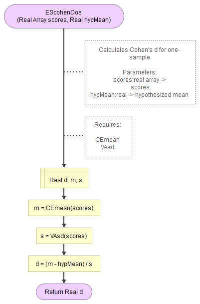
It takes as input paramaters the scores and the hypothesized mean.
It uses a function for the mean (CEmean), standard deviation (VAsd) which in turn use the MAsumReal function (sums array or real values).
Flowgorithm file: FL-EScohenDos.fprg.
with Python
Jupyter Notebook used in video: ES - Cohen d (one-sample).ipynb.
Data file used: GSS2012a.csv.
with R (Studio)
R script used in video: ES - Cohen's d (one-sample).R.
Datafile used in video: GSS2012-Adjusted.sav
with SPSS
This has become available in SPSS 27. As mentioned on this site, there is no option in earlier versions of SPSS to determine Cohen's D, but it can easily be calculated using by using the output from the t-test and entering the results below in the 'Online calculator' option, or using the 'Compute variable' option as shown in the video.
SPSS 27 or later
Datafile used in video: GSS2012-Adjusted.sav
SPSS 26 or earlier
Datafile used in video: GSS2012-Adjusted.sav
with an online calculator
Enter the sample mean, the hypothesized population mean, and the sample standard deviation:
manually (formula and example)
Formula's
The formula for Cohen's d for a one-sample t-test is:
\(d=\frac{\bar{x}-\mu_{H_{0}}}{s}\)
Where x̄ is the sample mean, μH0 the expected mean in the population (the mean according to the null hypothesis), and s the sample standard deviation.
The formula for the sample standard deviation is:
\(s=\sqrt{\frac{\sum_{i=1}^{n}\left(x_{i}-\bar{x}\right)^{2}}{n-1}}\)
In this formula xi is the i-th score, x̄ is the sample mean, and n is the sample size.
The sample mean can be calculated using:
\(\bar{x}=\frac{\sum_{i=1}^{n}x_{i}}{n}\)
Example (different example)
We are given the ages of five students, and have an hypothesized population mean of 24. The ages of the students are:
\(X=\left\{18,21,22,19,25\right\}\)
Since there are five students, we can also set n = 5, and the hypothesized population of 24 gives \(\mu_{H_{0}}=24\)
For the standard deviation, we first need to determine the sample mean:
\(\bar{x}=\frac{\sum_{i=1}^{n}x_{i}}{n}=\frac{\sum_{i=1}^{5}x_{i}}{5}=\frac{18+21+22+19+25}{5}\)
\(=\frac{105}{5}=21\)
Then we can determine the standard deviation:
\(s=\sqrt{\frac{\sum_{i=1}^{n}\left(x_{i}-\bar{x}\right)^{2}}{n-1}}=\sqrt{\frac{\sum_{i=1}^{5}\left(x_{i}-21\right)^{2}}{5-1}}=\sqrt{\frac{\sum_{i=1}^{5}\left(x_{i}-21\right)^{2}}{4}}\)
\(=\sqrt{\frac{\left(18-21\right)^{2}}{4}+\frac{\left(21-21\right)^{2}}{4}+\frac{\left(22-21\right)^{2}}{4}+\frac{\left(19-21\right)^{2}}{4}+\frac{\left(25-21\right)^{2}}{4}}\)
\(=\sqrt{\frac{\left(-3\right)^{2}}{4}+\frac{\left(0\right)^{2}}{4}+\frac{\left(1\right)^{2}}{4}+\frac{\left(-2\right)^{2}}{4}+\frac{\left(4\right)^{2}}{4}}\)
\(=\sqrt{\frac{9}{4}+\frac{0}{4}+\frac{1}{4}+\frac{4}{4}+\frac{16}{4}}=\sqrt{\frac{9+0+1+4+16}{4}}=\sqrt{\frac{30}{4}}\)
\(=\sqrt{\frac{15}{2}}=\frac{1}{2}\sqrt{15\times2}=\frac{1}{2}\sqrt{30}\approx2.74\)
Now for Cohen's d:
\(d=\frac{\bar{x}-\mu_{H_{0}}}{s}=\frac{21-24}{\frac{1}{2}\sqrt{30}}=\frac{-3}{\frac{\sqrt{30}}{2}}\)
\(=\frac{-3\times2}{\sqrt{30}}=\frac{-6}{\sqrt{30}}=\frac{-6}{\sqrt{30}}\times\frac{\sqrt{30}}{\sqrt{30}}=\frac{-6\times\sqrt{30}}{\sqrt{30}\times\sqrt{30}}\)
\(=\frac{-6\times\sqrt{30}}{30}=\frac{-6}{30}\times\sqrt{30}=-\frac{1}{5}\sqrt{30}\approx1.0954\)
Remember that this manual calculation was done using a different example.
For small sample sizes (when the sample size is less than 20), Cohen's d is a bit biased and can be corrected (Zaiontz, n.d.). This is then known as Hedges g. See below for more information on Hedges g (a.k.a. Hedges correction).
We've done enough analysing, so let's combine all the reports bit on the next section.
Click here for more info on Hedges g
Hedges g (Hedges, 1981) is a correction for Cohen's d that is needed for small sample size. It's calculation for larger samples becomes quite computational heavy, so approximations also exist for this.
Different authors have different definitions of 'small' but one example is n < 20 (Zaiontz, n.d.).
We could use the same table for interpretation, just don't forget to multiply the result with the square root of 2.
Click here to calculate Hedges g...
with Excel
Excel file: ES - Hedges g (one-sample).xlsm.
with Flowgorithm
A flowgorithm for Hedges g (one-sample) in Figure 1.

It takes as input paramaters the scores, the hypothesized mean, and which approximation to use (if any).
It uses a function for Cohen's d (EScohenDos), the gamma function (MAgamma), and the e power function (MAexp). Cohen's d function requires in turn the mean (CEmean) and standard deviation (VAsd) functions, which make use of the MAsumReal (sum of real values) function. The gamma function needs the factorial function (MAfact)
Flowgorithm file: FL-EShedgesGos.fprg.
with Python
Jupyter Notebook used in video: ES - Hedges g (one-sample).ipynb.
Data file used in video and notebook GSS2012a.csv.
with R (Studio)
video to be uploaded
R script: ES - Hedges g (one-sample).R.
Datafile used: GSS2012a.csv.
with SPSS
This has become available in SPSS 27. There is no option in earlier versions of SPSS to determine Hedges g, but it can easily be calculated using the 'Compute variable' option as shown in the video.
SPSS 27 or later
Datafile used in video: GSS2012-Adjusted.sav
SPSS 26 or earlier
Datafile used in video: GSS2012-Adjusted.sav
manually (Formula)
The exact formula for Hedges g is (Hedges, 1981, p. 111):
\(g = d\times\frac{\Gamma\left(m\right)}{\Gamma\left(m-0.5\right)\times\sqrt{m}}\)
With \(d\) as Cohen's d, and \(m = \frac{df}{2}\), where \(df=n-1\)
The \(\Gamma\) indicates the gamma function, defined as:
\(\Gamma\left(a=\frac{x}{2}\right)=\begin{cases} \left(a - 1\right)! & \text{ if } x \text{ is even}\\ \frac{\left(2\times a\right)!}{4^a\times a!}\times\sqrt{\pi} & \text{ if } x \text{ is odd}\end{cases}\)
Because the gamma function is computational heavy there are a few different approximations.
Hedges himself proposed (Hedges, 1981, p. 114):
\(g^* \approx d\times\left(1 - \frac{3}{4\times df-1}\right)\)
Durlak (2009, p. 927) shows another factor to adjust Cohens d with:
\(g^* = d\times\frac{n-3}{n-2.25}\times\sqrt{\frac{n-2}{n}}\)
Xue (2020, p. 3) gave an improved approximation using:
\(g^* = d\times\sqrt[12]{1-\frac{9}{df}+\frac{69}{2\times df^2}-\frac{72}{df^3}+\frac{687}{8\times df^4}-\frac{441}{8\times df^5}+\frac{247}{16\times df^6}}\)
Note 1. You might come across the following approximation: (Hedges & Olkin, 1985, p. 81)
\(g^* = d\times\left(1-\frac{3}{4\times n - 9}\right)\)
This is an alternative but equal method, but for the paired version. In the paired version we set df = n - 2, and if we substitute this in the Hedges version it gives the same result. The denominator of the fraction will then be:
\(4\times df - 1 = 4 \times\left(n-2\right) - 1 = 4\times n-4\times2 - 1 = 4\times n - 8 - 1 = 4\times n - 9\)
Note 2. Often for the exact formula 'm' is used for the degrees of freedom, and the formula will look like:
\(g = d\times\frac{\Gamma\left(\frac{m}{2}\right)}{\Gamma\left(\frac{m-1}{2}\right)\times\sqrt{\frac{m}{2}}}\)
Note 3: Alternatively the natural logarithm gamma can be used by using:
\(j = \ln\Gamma\left(m\right) - 0.5\times\ln\left(m\right) - \ln\Gamma\left(m-0.5\right)\)
and then calculate:
\(g = d\times e^{j}\)
In the formula for \(j\) we still use \(m = \frac{df}{2}\).
Single scale variable
![]()

Google adds