
Analysing a single nominal variable
are the percentages equal? (Pearson chi-square goodness-of-fit test)
Note: click here if you prefer to watch a video
One question you might have with a nominal variable, is if each category had the same number of respondents (i.e. the same percentage). With the marital status example from the previous paragraphs, we might expect each of the five categories to have (100% / 5 =) 20%. This would mean that we’d expected 20% of 1941 = 388.2 people in each category. This is known as the expected count or expected frequency.
Our observed frequencies are different from the expected ones. The Pearson chi-square test of goodness-of-fit (Pearson, 1900) can determine if the differences between the observed and expected counts is signficant. If the test result is a p-value below .05 it is usually considered signficant, indicating that there are some significant differences between some categories in frequencies.
One problem though is that the Pearson chi-square test of goodness-of-fit should only be used if not too many cells have a low so-called expected count. For this test it is usually set that all cells should have an expected count of at least 5 (see for example Peck & Devore, 2012, p. 593) (note that for a Pearson chi-square test of independence the conditions are different). If you don't meet this criteria, you could use an exact multinomial test of goodness-of-fit. This test is explained in the appendix at the bottom of this page. McDonald (2022) even suggests to always use this exact test as long as the sample size is less than 1000 (which was just picked as a nice round number, when n is very large the exact test becomes computational heavy even for computers).
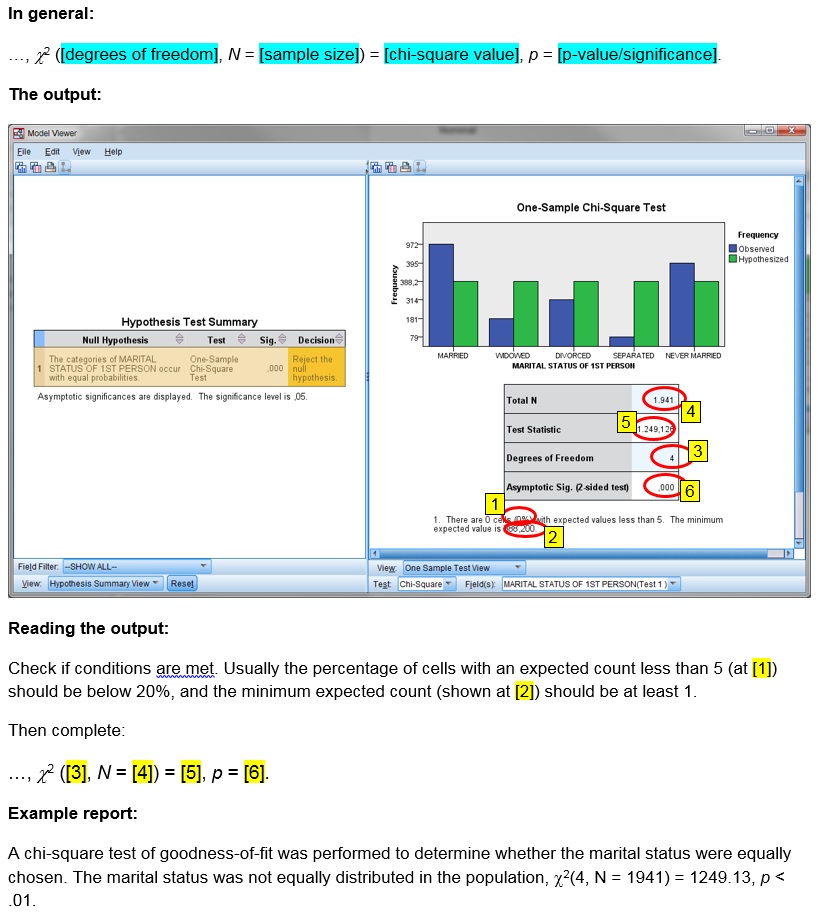
Once you have checked the conditions and looked at the results, you can report the test results. You will need the significance, but also the chi-square value itself, the sample size (number of respondents that answered this question), and the so-called degrees of freedom. This last one is simply for this test the number of categories minus 1. In the example the percentage of cells with an expected count less than 5 is actually 0%, so it is okay to use the test. The test results showed that the sig. was .000. This indicates it was less than .0005 and is then often reported simply as < .001. We had five categories, so the degrees of freedom is 5 – 1 = 4, the sample size was 1941 and the chi-square value (calculated by the software) was 1249.13. The test results could then be reported as something like
A chi-square test of goodness-of-fit was performed to determine whether the marital status were equally chosen. The marital status was not equally distributed in the population, χ2(4, N = 1941) = 1249.13, p < .001.
Click here to see how to perform a Pearson chi-square goodness-of-fit test
with Excel
Excel file from video: TS - Pearson chi-square GoF.xlsm.
with Flowgorithm
A basic implementation for Pearson Chi-Square GoF test in the flowchart in figure 1
Figure 1
Flowgorithm for the Pearson Chi-Square GoF test
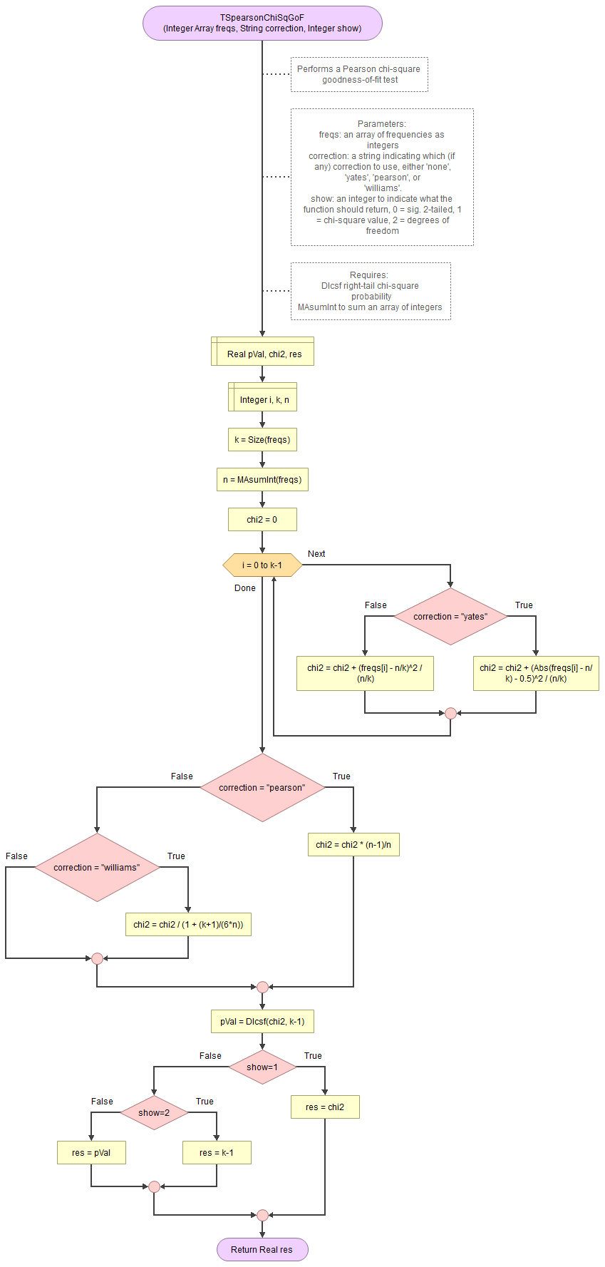
It takes as input an array of integers with the observed frequencies, a string to indicate which correction to use (either 'none', 'pearson', 'williams', or 'yates') and an integer for which output to show (0 = sig., 1=chi-square value, 2 = degrees of freedom).
It uses the function for the right-tail probabilities of the chi-square distribution and a small helper function to sum an array of integers.
Flowgorithm file: FL-TSpearsonChiSqGoF.fprg.
with Python
Jupyter Notebook from video: TS - Pearson chi-square GoF.ipynb.
Data file from video: GSS2012a.csv.
with R (Studio)
Click or hover over the thumbnail below to see where to look in the output.

R script from video: TS - Pearson chi-square GoF.R.
Data file from video: Pearson Chi-square independence.csv.
with SPSS
via One-sample
Click or hover over the thumbnail below to see where to look in the output.
Data file used in video: GSS2012-Adjusted.sav.
via Legacy dialogs
Click or hover over the thumbnail below to see where to look in the output.

Data file used in video: GSS2012-Adjusted.sav.
Manually (Formula and example)
The formula's
The Pearson chi-square goodness-of-fit test statistic (χ2):
\( \chi^{2}=\sum_{i=1}^{k}\frac{\left(O_{i}-E_{i}\right)^{2}}{E_{i}}\)
In this formula Oi is the observed count in category i, Ei is the expected count in category i, and k is the number of categories.
If the expected frequencies, are expected to be equal, then:
\(E_{i}=\frac{\sum_{j=1}^{k}O_{i}}{k}\)
The degrees of freedom is given by:
\(df=k-1\)
The probability of such a chi-square value or more extreme, can then be found using the chi-square distribution.
Example
We have the following observed frequencies of five categories:
\(O=\left(972,181,314,79,395\right)\)
Note that since there are five categories, we have k = 5. If the expected frequency for each category is expected to be equal we can use the formula to determine:
\(E_{i}=\frac{\sum_{j=1}^{k}O_{i}}{k}=\frac{\sum_{j=1}^{5}O_{i}}{5} =\frac{972+181+314+79+395}{5}\)
\(=\frac{1941}{5}=388\frac{1}{5}=388.2\)
Then we can determine the Pearson chi-square value:
\(\chi^{2}=\sum_{i=1}^{k}\frac{\left(O_{i}-E_{i}\right)^{2}}{E_{i}}=\sum_{i=1}^{5}\frac{\left(O_{i}-\frac{1941}{5}\right)^{2}}{\frac{1941}{5}}\)
\(=\frac{\left(972-\frac{1941}{5}\right)^{2}}{\frac{1941}{5}}+\frac{\left(181-\frac{1941}{5}\right)^{2}}{\frac{1941}{5}}+\frac{\left(314-\frac{1941}{5}\right)^{2}}{\frac{1941}{5}}+\frac{\left(79-\frac{1941}{5}\right)^{2}}{\frac{1941}{5}}+\frac{\left(395-\frac{1941}{5}\right)^{2}}{\frac{1941}{5}}\)
\(=\frac{\left(\frac{972\times5}{5}-\frac{1941}{5}\right)^{2}}{\frac{1941}{5}}+\frac{\left(\frac{181\times5}{5}-\frac{1941}{5}\right)^{2}}{\frac{1941}{5}}+\frac{\left(\frac{314\times5}{5}-\frac{1941}{5}\right)^{2}}{\frac{1941}{5}}+\frac{\left(\frac{79\times5}{5}-\frac{1941}{5}\right)^{2}}{\frac{1941}{5}}+\frac{\left(\frac{395\times5}{5}-\frac{1941}{5}\right)^{2}}{\frac{1941}{5}}\)
\(=\frac{\left(\frac{972\times5-1941}{5}\right)^{2}}{\frac{1941}{5}}+\frac{\left(\frac{181\times5-1941}{5}\right)^{2}}{\frac{1941}{5}}+\frac{\left(\frac{314\times5-1941}{5}\right)^{2}}{\frac{1941}{5}}+\frac{\left(\frac{79\times5-1941}{5}\right)^{2}}{\frac{1941}{5}}+\frac{\left(\frac{395\times5-1941}{5}\right)^{2}}{\frac{1941}{5}}\)
\(=\frac{\left(\frac{4860-1941}{5}\right)^{2}}{\frac{1941}{5}}+\frac{\left(\frac{905-1941}{5}\right)^{2}}{\frac{1941}{5}}+\frac{\left(\frac{1570-1941}{5}\right)^{2}}{\frac{1941}{5}}+\frac{\left(\frac{395-1941}{5}\right)^{2}}{\frac{1941}{5}}+\frac{\left(\frac{1975-1941}{5}\right)^{2}}{\frac{1941}{5}}\)
\(=\frac{\left(\frac{2919}{5}\right)^{2}}{\frac{1941}{5}}+\frac{\left(\frac{-1036}{5}\right)^{2}}{\frac{1941}{5}}+\frac{\left(\frac{-371}{5}\right)^{2}}{\frac{1941}{5}}+\frac{\left(\frac{-1546}{5}\right)^{2}}{\frac{1941}{5}}+\frac{\left(\frac{34}{5}\right)^{2}}{\frac{1941}{5}}\)
\(=\frac{\frac{\left(2919\right)^{2}}{5^{2}}}{\frac{1941}{5}}+\frac{\frac{\left(-1036\right)^{2}}{5^{2}}}{\frac{1941}{5}}+\frac{\frac{\left(-371\right)^{2}}{5^{2}}}{\frac{1941}{5}}+\frac{\frac{\left(-1546\right)^{2}}{5^{2}}}{\frac{1941}{5}}+\frac{\frac{\left(34\right)^{2}}{5^{2}}}{\frac{1941}{5}}\)
\(=\frac{\frac{8520561}{5^{2}}}{\frac{1941}{5}}+\frac{\frac{1073296}{5^{2}}}{\frac{1941}{5}}+\frac{\frac{137641}{5^{2}}}{\frac{1941}{5}}+\frac{\frac{2390116}{5^{2}}}{\frac{1941}{5}}+\frac{\frac{1156}{5^{2}}}{\frac{1941}{5}}\)
\(=\frac{8520561\times5}{1941\times5^{2}}+\frac{1073296\times5}{1941\times5^{2}}+\frac{137641\times5}{1941\times5^{2}}+\frac{2390116\times5}{1941\times5^{2}}+\frac{1156\times5}{1941\times5^{2}}\)
\(=\frac{8520561}{1941\times5}+\frac{1073296}{1941\times5}+\frac{137641}{1941\times5^{2}}+\frac{2390116}{1941\times5}+\frac{1156}{1941\times5}\)
\(=\frac{8520561+1073296+137641+2390116+1156}{1941\times5}\)
\(=\frac{12122770}{1941\times5}=\frac{2424554\times5}{1941\times5}=\frac{2424554}{1941}\approx1249.13\)
The degrees of freedom is:
\(df=k-1=5-1=4\)
To determine the signficance you then need to determine the area under the chi-square distribution curve, in formula notation:
\(\int_{x=0}^{\chi^{2}}\frac{x^{\frac{df}{2}-1}\times e^{-\frac{x}{2}}}{2^{\frac{df}{2}}\times\Gamma\left(\frac{df}{2}\right)}\)
This is usually done with the aid of either a distribution table, or some software. See the chi-square distribution section for more details.
The Pearson Chi-square goodness-of-fit test is actually a so-called omnibus test, it tests all categories in one time. Unfortunately because of this, it does not inform us when it is significant, which categories are significantly different. How to determine this, is discussed in the next part.
Besides the exact multinomial test there are many other alternatives. The so-called G-test, or sometimes called likelihood-ratio test or Wilks test has as an advantage of a that the results are so-called additive, which means they could be combined with other results in larger studies, the disadvantage is that it is a far less familiar test than the Pearson version (McDonald, 2014).
Besides chosing a test, there are also various corrections for chi-square tests. More on these corrections can be found in the appendix.
In short the Pearson chi-square test of goodness-of-fit has the following steps:
- The assumption about the population (the null hypothesis (H0)) is that the observed and expected counts will be the same. This implies that the two variables are independent (i.e. one has no influence on the other).
- The alternative is that they aren't (Ha). This implies that the two variables are dependent (i.e. one has an influence on the other)
- Perform the test and find the p-value (sig.).
- If the p-value is less than .05, the chance of a result as in the sample or even rarer if the assumption is true, is considered so low, that the assumption is probably NOT true. We would then reject H0 and conclude Ha. This is then called a significant result.
- If the p-value is .05 or more, the chance of a result as in the sample or even rarer if the assumption is true, is considered not low enough, that the assumption could be true. We don't have enough evidence to reject the assumption. This is then called a non-significant result.
Appendix
Click here to see how to perform an Exact Multinomial Goodness-of-Fit test
If you do not meet the criteria, there are three options. First off, are you sure you have a nominal variable, and not an ordinal one? If you have an ordinal variable, you probably want a different test. If you are sure you have a nominal variable you might be able to combine two or more categories into one larger category. If for example you asked people about their country of birth, but a few countries were only selected by one or two people, you might want to combine these simply into a category ‘other’. Be very clear though in your report that you’ve done so. Another option is to use a so called exact-multinomial test. This test does not have the criteria but will need larger differences before it will actually determine some of them to be significant.
with Excel
Excel file from video: TS - Exact Multinomial GoF.xlsm.
with Python
Jupyter Notebook from video TS - Exact Multinomial GoF (Python).ipynb.
Datafile used StudentStatistics.csv.
with R (Studio)
Jupyter Notebook from video TS - Exact Multinomial GoF (R).ipynb.
Datafile used StudentStatistics.csv.
with SPSS
Datafile used StudentStatistics.sav.
Manually
To calculate the exact multinomial test by hand the following steps can be used.
Step 1: Determine the probability of the observed counts using the probability mass function of the multinomial distribution.
The formula for this is given by:
\(\frac{n!}{\prod_{i=1}^{k}F_i!}\times\prod_{i=1}^{k}\pi_i^{F_i}\)
Where \(n\) is the total sample size, \(k\) the number of categories, \(F_i\) the frequency of the i-th category, and \(\pi_i\) the expected proportion of the i-th category.
Step 2: Determine all possible permutations with repetition that create a sum equal to the sample size over the k-categories.
Step 3: Determine the probability of each of these permutations using the probability mass function of the multinomial distribution.
Step 4: Sum all probabilities found in step 3 that are equal or less than the one found in step 1.
Step 2 is quite tricky. We could create all possible permutations with replacement. If our sample size is n and the number of categories is k, this gives \((n+1)^k\) permutations. The ‘+ 1’ comes from the option of 0 to be included. Most of these permutations will not sum to the sample size, so they can be removed.
If the expected probability for each category is the same, we could use another approach. We could then create all possible combinations with replacement. This would give fewer results:
\(\binom{n+k}{k}=\frac{(n+k)!}{n!k!}\)
Again we can then remove the ones that don’t sum to the sample size. Then perform step 3, but now multiply each by how many variations this can be arranged in. If for example we have 5 categories, and a total sample size of 20, one possible combination is [2, 2, 3, 3, 10]. This would be the same as [2, 3, 3, 2, 10], [2, 3, 10, 2, 3], etc. We could determine the count (frequency) of each unique score, so in the example 2 has a frequency of 2, 3 also and 10 only one. Now the first 2 we can arrange in:
\(\binom{5}{2}=\frac{5!}{(5-2)!2!}=10\)
The 5 is our number of categories, the 2 the frequency. For the two 3’s we now have 5 – 2 = 3 spots left, so those can only be arranged in:
\(\binom{3}{2}=\frac{3!}{(3-2)!2!}=3\)
Combining these 3 with the 10 we had earlier gives 3×10=30 possibilities. The single 10 only can now go to one spot so that’s it.
In general, if we have k categories, m different values and F_i is the i-th frequency of those values, sorted from high to low, we get:
\(\binom{k}{F_1}\prod_{i=2}^m\binom{k-\sum_{j=1}^{m-i+1}F_j}{F_j}=\binom{k}{F_1}\binom{k-F_1}{F_2}\binom{k-\sum_{j=1}^{2}F_j}{F_3}…\binom{k-\sum_{j=1}^{m-1}F_j}{F_k}\)
Where:
\(\binom{a}{b}=\frac{a!}{(a-b)!b!}\)
Click here to see how you can perform a Likelihood Ratio Goodness-of-Git test (G-test of GoF, Wilks test of Gof).
with Excel
Excel file: TS - G-test (GoF).xlsm.
with Flowgorithm
A basic implementation for G-test of GoF in the flowchart in figure 1
Figure 1
Flowgorithm for the G-test of GoF
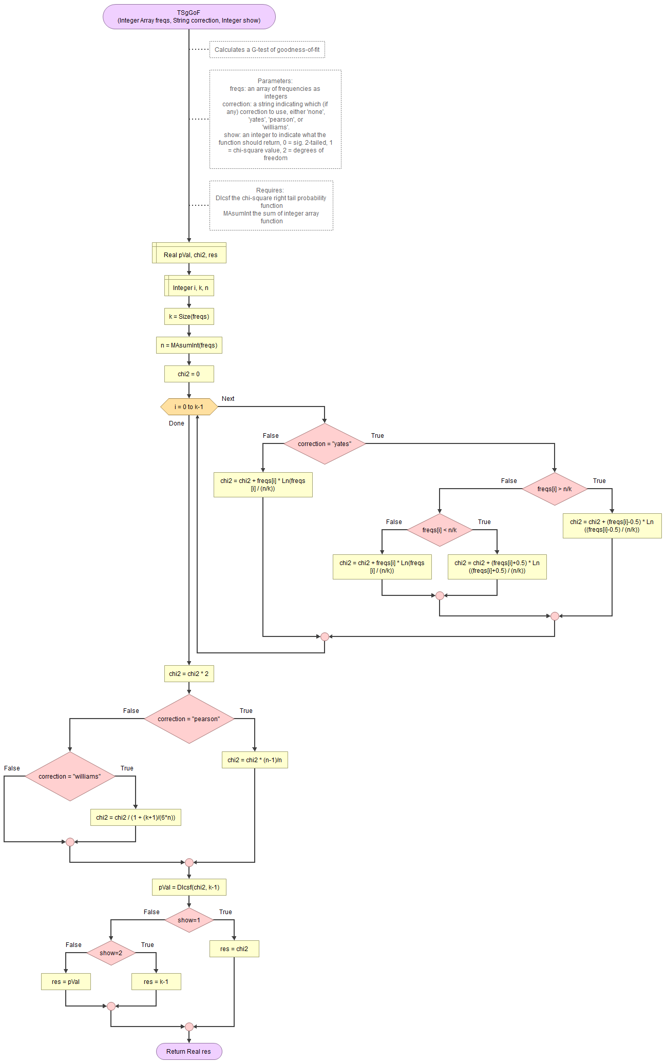
It takes as input an array of integers with the observed frequencies, a string to indicate which correction to use (either 'none', 'pearson', 'williams', or 'yates') and an integer for which output to show (0 = sig., 1=chi-square value, 2 = degrees of freedom).
It uses the function for the right-tail probabilities of the chi-square distribution and a small helper function to sum an array of integers.
Flowgorithm file: FL-TSgGoF.fprg.
Manually
In the formula's the following variables will be used:
Oi is the observed count in category i
Ei is the expected count in category i
k is the number of categories
The likelihood-ratio goodness-of-fit test statistic (G):
\(G=2\times\sum_{i=1}^{k}\left(O_{i}\times ln\left(\frac{O_{i}}{E_{i}}\right)\right)\)
The degrees of freedom (df):
\(df=k-1\)
The G-value follows a chi-square distribution. To determine the signficance you then need to determine the area under the chi-square distribution curve, in formula notation:
\(\int_{x=0}^{\chi^{2}}\frac{x^{\frac{df}{2}-1}\times e^{-\frac{x}{2}}}{2^{\frac{df}{2}}\times\Gamma\left(\frac{df}{2}\right)}\)
This is usually done with the aid of either a distribution table, or some software. See the chi-square distribution section for more details.
Corrections for the chi-square test
The chi-square distribution is a so-called continuous distribution. This means it accepts decimal values as input. However, since we are testing frequencies, these cannot be having a decimal value, and hence the exact multinomial test uses a discrete distribution. To compensate for this a few different corrections exist.
The first is known as the Yates continuity correction. It adjusts the chi-square value in the calculation itself by adding or subtracting 0.5, depending on if the frequency or the expected frequency is higher (Yates, 1934, p. 222). This is actually the same as subtracting 0.5 from the absolute difference, since we are squaring the results anyway after. In formula notation the Yates correction for a Pearson chi-square GoF test can be written as:
\(\chi_{Yates}^{2} = \sum_{i=1}^{k}\frac{\left(\left|F_i - E_i\right|-0.5\right)^2}{E_i}\)
In this formula \(k\) is the number of categories, \(F_i\) the observed frequency of category i, and \(E_i\) the expected frequency of category i.
For a G-test GoF the correction goes slightly different:
\(\chi_{G-Yates}^2 = 2\times \sum_{i=1}^k\left(F_i^{'}\times ln\left(\frac{F_i^{'}}{E_i}\right)\right)\)
with: \(F_i^{'}=\begin{cases} F_i-0.5 & \text{ if } F_i > E_i \\ F_i+0.5 & \text{ if } F_i\lt E_i \\ F_i & \text{ if } F_i=E_i\end{cases} \)
Note however, that this correction is usually only recommended if the degrees of freedom is two. For a goodness-of-fit test this means only if you have two categories.
The E.S. Pearson correction simply adjusts the chi-square value by multiplying it with \(\frac{n-1}{n}\) (E.S. Pearson, 1947, p. 157). Note that this is a different Pearson than the one from the Pearson chi-square test itself. The correction in formula notation:
\(\chi_{E.Pearson}^{2} = \chi^2 \times \frac{n-1}{n}\)
A third correction is from Williams (1976). This suggests to divide the chi-square value by a specific value \(q\), which for a goodness-of-fit test is defined as:
\(q = 1 + \frac{k^2-1}{6\times n\times df}\)
In this formula \(k\) is the number of categories, \(n\) the sample size, and \(df\) the number of categories minus one, i.e. \(df=k-1\) (unless you have an intrinsic null hypothesis). After the calculation of \(q\) the corrected chi-square value is:
\(\chi_{Williams}^2=\frac{\chi^2}{q}\)
If indeed \(df=k-1\) the formula for \(q\) can be simplified to:
\(q = 1 + \frac{k+1}{6\times n}\)
Single nominal variable
![]()

Google adds